Mastering CFG: Diagnosis and Artifacts

1. The Guidance Scale Trade-Off: Fidelity vs. Diversity

The guidance scale, $s$, fundamentally controls a trade-off between fidelity (how closely the output adheres to the condition) and diversity (the variety and, often, the perceptual quality of the outputs).

• Low Scale ($s\approx 1-4$): The guidance is weak. The model generates diverse samples that are close to its learned data distribution, but they might not follow the condition very precisely. Think of it as giving the model a gentle suggestion.
• Medium Scale ($s\approx 5-10$): This range often represents a "sweet spot." It provides a good balance where the model strongly adheres to the condition while maintaining high perceptual quality and reasonable diversity. Many text-to-image models use a default around 7.5.
• High Scale ($s>10$): The guidance is very strong. The model is forced to generate samples that are "extremely" representative of the condition. This can improve prompt adherence but often comes at a cost.

This trade-off can be measured quantitatively. Fidelity to a text prompt is often measured by CLIP Score, while overall sample quality and diversity are measured by metrics like Fréchet Inception Distance (FID). As you might expect from your experience with similar trade-offs in ML, increasing the CFG scale generally improves the CLIP score up to a point, but eventually degrades the FID score.

2. Diagnosing Artifacts of High Guidance

When you push the guidance scale too high, you are essentially extrapolating far outside the data distribution the model was trained on. This leads to several common visual artifacts that you should learn to recognize.

As the article notes, the primary artifacts to watch for are:

1. Intensity Oversaturation: This is the most common issue. Colors become unnaturally bright and clipped, leading to flat, blown-out areas in the image. This happens because the guidance pushes predicted pixel values beyond the valid normalized range (e.g., [-1, 1]).
2. Out-of-Distribution Samples: The images can look strange or unrealistic. Details might become distorted, textures can appear artificial, and the overall composition can feel simplified or "cartoonish." The model is generating an "easy-to-classify" image that perfectly matches the condition from a mathematical perspective but looks wrong to a human eye.
3. Limited Diversity: At very high scales, the model tends to produce very similar outputs for the same prompt, collapsing into a few stereotypical modes.

3. Mitigation Strategy 1: Dynamic Thresholding

Since oversaturation is caused by pixel values exceeding their valid range, a direct solution is to force them back. This is the idea behind thresholding.

To summarize the key ideas from the reading:

• The Problem: The CFG update step can push the predicted denoised image ${\hat{x}}_0$ to have values outside the [-1, 1] range. When this happens repeatedly over many steps, the final image becomes saturated.
• Static Thresholding: A simple fix. After each guidance step, you clamp the predicted ${\hat{x}}_0$ values to be within [-1, 1]. This helps but can be too aggressive, losing some image detail.
• Dynamic Thresholding: A smarter approach. Instead of clamping to a fixed [-1, 1], you determine a dynamic threshold, $s$, at each step. This $s$ is typically set to a high percentile (e.g., 99.5%) of the absolute pixel values in the current ${\hat{x}}_0$. You then clip the values to [-s, s] and rescale the entire image by dividing by $s$. This preserves more dynamic range while preventing extreme saturation.

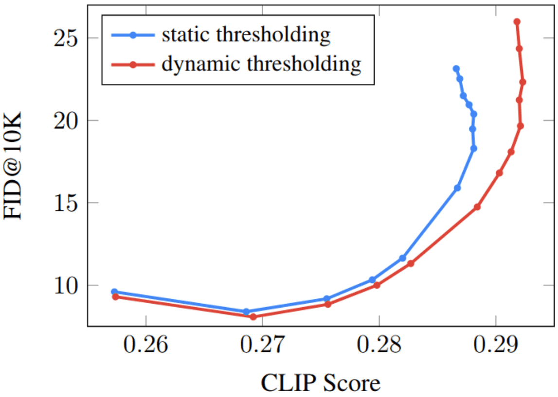
Dynamic thresholding is a relatively simple addition to your sampling loop that can significantly expand the usable range of your CFG scale.

4. Mitigation Strategy 2: Advanced Guidance Schedules

Another line of attack is to recognize that the optimal guidance strength may not be constant throughout the entire denoising process. Recent research has shown that applying strong guidance can be harmful in the early, high-noise steps and less impactful in the final, low-noise steps.

The key takeaway is the concept of Limited Interval CFG. Instead of applying guidance at every step, you only apply it in an intermediate range of noise levels (${\sigma }_{low}<\sigma <{\sigma }_{high}$).

• Early Steps (high noise $\sigma$): No guidance ($s=1$). This allows the model to form the basic structure of the image without being pushed off-distribution by a noisy guidance signal.
• Middle Steps (intermediate $\sigma$): Apply guidance ($s>1$). This is where guidance is most effective, refining the image to match the condition.
• Late Steps (low noise $\sigma$): No guidance ($s=1$). At this stage, the main details are set, and guidance has less impact.

This approach requires hyperparameter tuning for the interval boundaries but can significantly improve the final FID score by preventing the sampling trajectory from drifting too far from the learned data manifold.

5. Mitigation Strategy 3: Adaptive Projected Guidance (APG)

Recently, researchers have developed more principled methods to disentangle the positive and negative effects of CFG. One of the most promising is Adaptive Projected Guidance (APG). Given your background, the vector decomposition at the heart of this method should be quite intuitive.

The core idea is to decompose the CFG update vector, $\Delta D_t=D_{\theta }(z_t,t,y)-D_{\theta }(z_t,t,y_{null})$, into two components:

1. A component parallel to the conditional prediction $D_{\theta }(z_t,t,y)$.
2. A component orthogonal to the conditional prediction.

The key insight is that the parallel component is primarily responsible for oversaturation, while the orthogonal component is what improves image quality and detail. APG leverages this by down-weighting the parallel component.

APG combines three ideas:

• Projection: It reduces the strength of the parallel component of the guidance vector, directly combating saturation.
• Rescaling: It normalizes the guidance update to prevent excessively large steps, inspired by normalized gradient ascent methods.
• Reverse Momentum: It uses a momentum term with a negative value, encouraging the model to explore new update directions at each step rather than reinforcing previous ones.

As the paper demonstrates, APG allows for the use of very high guidance scales to maximize prompt adherence without the usual penalty of oversaturation and artifacts, making it a superior plug-and-play alternative to standard CFG.

Conclusion

You've now moved beyond simply using CFG to understanding how to master it. This is a critical skill for producing state-of-the-art results with diffusion models.

Key Takeaways:

• CFG involves a trade-off: Tuning the guidance scale, $s$, is a balancing act between fidelity to the condition and the overall diversity and quality of the generated image.
• High guidance has known failure modes: Be prepared to diagnose common artifacts like color oversaturation, simplified compositions, and a general lack of realism.
• You have a toolbox of mitigation strategies:
  • Dynamic Thresholding is a simple and effective fix for oversaturation, applied within the sampling loop.
  • Guidance Scheduling (like Limited Interval CFG) offers a more nuanced approach by making the guidance strength dependent on the noise level.
  • Adaptive Projected Guidance (APG) provides a principled, state-of-the-art solution by decomposing the guidance vector to isolate and reduce the component that causes saturation.

Next Lesson Preview:

So far, our conditioning has been based on simple class labels. The real power of modern diffusion models comes from using complex text prompts. But what happens when the model seems to ignore part of your prompt? Simply cranking up the CFG scale often isn't the right answer. In our next lesson, we will begin to look inside the U-Net and learn to analyze cross-attention maps to debug prompt alignment failures. This will be our first step toward understanding and controlling the intricate relationship between text and image generation.