Class Conditioning with Learned Embeddings

1. The Core Idea: From Class Index to Learnable Embedding

Just as we couldn't feed the raw timestep integer $t$ directly into our U-Net, we can't simply use a class index like 3 as a direct input. The model needs a richer, higher-dimensional representation that it can learn to associate with the visual features of that class.

The standard solution is to use a learnable embedding layer. In PyTorch, this is torch.nn.Embedding. It acts as a simple lookup table:

• It is initialized as a matrix of size (num_classes, embedding_dim).
• When you pass it an integer (the class index), it returns the corresponding row from the matrix—a dense vector representing that class.
• Crucially, these vectors are parameters of the model and are updated via backpropagation during training. The model learns to create meaningful representations for each class.

The diagram below illustrates this concept. The class label $y$ is fed into an "Embed Net" (which in our case is the nn.Embedding layer) to produce a conditioning vector $h_y$. This vector, along with the time embedding, is then used to condition the U-Net.

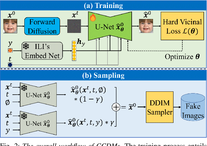
2. Integration Strategy 1: Additive Conditioning

Once we have our class embedding vector, how do we inject it into the U-Net? The most common and straightforward method is to add it to the timestep embedding.

Think of the sinusoidal timestep embedding as creating a "conditioning bus" that is already wired to various blocks within the U-Net. By simply adding our class embedding to the time embedding, we are placing our new conditioning signal onto this existing bus. It's an efficient way to distribute the class information throughout the network.

The following video provides a very clear and concise walkthrough of the code changes required to implement this.

To summarize the key modifications for this additive approach:

1. In the U-Net's __init__ method:

   • Accept a num_classes argument.
   • Define the embedding layer: self.label_emb = nn.Embedding(num_classes, time_emb_dim). The embedding dimension should match the timestep embedding dimension to allow for addition.

2. In the U-Net's forward method:

   • Accept an optional labels argument.
   • Compute the time embedding as usual.
   • If labels are provided, compute the label embedding: label_emb = self.label_emb(labels).
   • Add the two embeddings: time_emb = time_emb + label_emb.

3. In the training loop:

   • Ensure your data loader yields both images and their corresponding class labels.
   • Pass the labels batch to the model during the forward pass: output = model(x, t, labels).

3. Enabling Unconditional Generation: Dropping Labels

A powerful conditional model should ideally also be capable of generating images unconditionally. This capability is the foundation for an important technique called Classifier-Free Guidance (CFG), which we will cover in the next lesson.

To train a single model to do both, we use a simple but effective trick during training: we randomly "drop" the conditioning information for a fraction of the training samples. This forces the model to learn to denoise the image even when no class label is provided.

There are two common ways to implement this "label dropout":

1. Add a "null" class: Augment your dataset to have K+1 classes, where the last class represents "unconditional." During training, randomly replace a certain percentage of true labels with this null class index.
2. Use a zero vector (for one-hot encoding): If you represent your labels as one-hot vectors, dropping the label can be implemented by simply passing an all-zero vector. This is an elegant way of telling the model "no class information is available for this sample."

The following video explains this concept and then provides a complete code walkthrough.

Now, let's see how this is put into practice in an end-to-end implementation.

4. Integration Strategy 2: Multiplicative Modulation

An alternative to adding the class embedding to the time signal is to use it to directly modulate the feature maps within the U-Net. A common way to do this is with Feature-wise Linear Modulation (FiLM), where the conditioning embedding is used to predict a scaling factor ($\gamma$) and a shifting factor ($\beta$) that are applied to the normalized feature maps: output = (γ * normalized_features) + β.

A simpler variant just uses scaling. This allows the class information to control the "gain" of different features at various points in the network, potentially offering more fine-grained control than simple additive conditioning.

The Neuromatch tutorial provides a great implementation of this multiplicative scaling approach.

Choosing between additive and multiplicative conditioning is an architectural decision. Additive is simpler and often works very well. Multiplicative modulation can offer more expressive control over features and is a common pattern in conditional generative models.

def forward(self, x, t, y = None):
    # Obtain the Gaussian random feature embedding for t
    embed = self.act(self.time_embed(t))
    y_embed = self.cond_embed(y)

    # Encoding path
    h1 = self.conv1(x) + self.t_mod1(embed)
    h1 = self.act(self.gnorm1(h1))
    
    h2 = self.conv2(h1) + self.t_mod2(embed)
    h2 = h2 * self.y_mod2(y_embed) # <-- Multiplicative modulation
    h2 = self.act(self.gnorm2(h2))
    # ... and so on

def forward(self, x, t, y = None):
    # Obtain the Gaussian random feature embedding for t
    embed = self.act(self.time_embed(t))

    # --- MODIFICATION START ---
    # Add class embedding to time embedding if 'y' is provided
    if y is not None:
        y_embed = self.cond_embed(y)
        embed = embed + y_embed
    # --- MODIFICATION END ---
    
    # Encoding path
    h1 = self.conv1(x) + self.t_mod1(embed) # 'embed' now contains time + class info
    h1 = self.act(self.gnorm1(h1))
    
    h2 = self.conv2(h1) + self.t_mod2(embed) # 'embed' now contains time + class info
    # h2 = h2 * self.y_mod2(y_embed) # <-- This line is removed
    h2 = self.act(self.gnorm2(h2))
    # ... and so on

Conclusion

In this lesson, you've learned how to add class conditioning to your diffusion model, a fundamental step towards creating more controllable generative systems.

Key Takeaways:

• Learned Embeddings: Class indices are mapped to dense, learnable vectors using an nn.Embedding layer.
• Integration Strategies: These embeddings can be injected into the U-Net either by adding them to the timestep embeddings or by multiplicatively modulating the feature maps.
• Label Dropping: Randomly dropping class labels during training is a crucial technique that forces the model to learn to generate unconditionally. This is the key prerequisite for classifier-free guidance.

Next Lesson Preview:

We have now perfectly set the stage for one of the most significant improvements in diffusion model sampling. With a model trained to make both conditional and unconditional predictions, we can combine these at inference time to amplify the conditioning signal. In the next lesson, we will explain the mechanism of classifier guidance and implement classifier-free guidance (CFG). You'll see how this technique dramatically improves sample quality and adherence to the given condition.