Gradient Checkpointing for Memory Reduction

1. Understanding Memory Usage in Neural Network Training

Before we can reduce memory consumption, we need to understand where it's all going. When you train a large model like a diffusion U-Net, the memory on your GPU is consumed by several key components.

To get a clear breakdown, let's start with a reading that explains the two primary types of memory usage.

As you just read, the total memory can be broken down as follows:

• Static Memory: This is relatively fixed once training starts. It includes:

  • Model Weights: The parameters of your network.
  • Optimizer States: Adam/AdamW optimizers store running averages (mean and variance of gradients), which effectively doubles the memory required for trainable parameters.
  • Gradients: A gradient must be stored for every model parameter.

• Dynamic Memory: This is the part that fluctuates during the forward and backward passes. The main component is the activations (the outputs of each layer) that are saved during the forward pass. PyTorch's autograd engine stores these in a computation graph because they are needed to calculate the gradients during the backward pass. This dynamic memory usage scales with both the model's depth/complexity and, crucially, the batch size.

It is this dynamic memory, the stored activations, that often becomes the bottleneck and is the specific target of gradient checkpointing.

2. The Gradient Checkpointing Trade-Off

So, if storing activations is the problem, what's the solution? The core idea of gradient checkpointing is simple but powerful: don't store everything; recompute it when needed.

Instead of saving the output of every single layer during the forward pass, we strategically "forget" most of them. We only save the inputs to certain "checkpointed" segments of our model. Then, during the backward pass, when PyTorch needs an activation that was forgotten, it temporarily re-runs the forward pass for that small segment to regenerate it, uses it to compute the gradient, and then discards it again.

This is a classic computer science trade-off:

• We save memory: by not storing the intermediate activations for the entire batch.
• We spend compute: by performing a second, partial forward pass during backpropagation.

The image below provides an excellent visual conceptualization of this process.

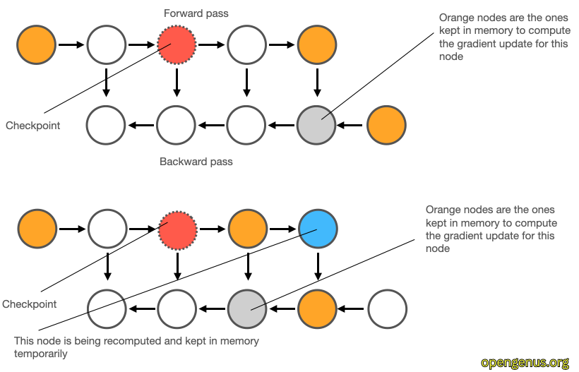
Let's read a more detailed explanation of how this works and the benefits it provides.

As the benchmarks show, the impact is significant. A ~60% reduction in peak memory for a ~25% increase in training time is often a fantastic trade-off, as it can be the difference between a training run succeeding or failing with an out-of-memory (OOM) error. It can also allow you to increase your batch size, which can improve gradient quality and speed up convergence.

3. Applying Gradient Checkpointing in Code

Now let's move to the practical application. PyTorch provides built-in utilities for gradient checkpointing, and high-level libraries like Hugging Face transformers and accelerate make it even simpler.

3.1. Using torch.utils.checkpoint

The most flexible way to apply gradient checkpointing is by using torch.utils.checkpoint.checkpoint to wrap specific modules within your model's forward method. This gives you fine-grained control over which parts of the network trade compute for memory.

The resource below provides the essential code patterns and, more importantly, highlights critical caveats you must be aware of as a practitioner.

Let's summarize the key implementation points:

1. Wrapping a Module: You replace a standard module call like X = self.cnn_block_2(X) with X = checkpoint(self.cnn_block_2, X).
2. Strategic Placement: You should apply checkpointing to the most memory-intensive parts of your network. In a U-Net, the large convolutional blocks in the middle and decoder path are excellent candidates.
3. Handling Non-Deterministic Layers: This is a crucial point. Gradient checkpointing performs a second forward pass. If a layer behaves differently on this second pass, the recomputed activations won't match the original ones, leading to incorrect gradients.
   • nn.Dropout is the classic example. It will randomly drop different neurons on the second pass.
   • nn.BatchNorm in training mode also poses a problem as its running statistics would be updated twice.
   • Solution: Refactor your model to pull these layers out of the checkpointed segment. In the example you read, dropout_2 is applied after the checkpointed cnn_block_2.

3.2. Using High-Level Frameworks

Modern training libraries make this even easier. If you are using a model from the Hugging Face ecosystem, or using their accelerate library for your own custom training loop, enabling gradient checkpointing is often a one-line change.

This model.gradient_checkpointing_enable() call is particularly powerful. For compatible models (like the standard U-Net in diffusers), it automatically and intelligently applies checkpointing to the appropriate blocks (e.g., the AttnDownBlock2D, AttnUpBlock2D, etc.) without you needing to modify the forward pass manually.

# A simplified U-Net forward pass
def forward(self, x, t):
    # ... initial conv ...

    # Down-sampling blocks
    x = self.down_block_1(x, t)
    x = self.down_block_2(x, t)
    x = self.down_block_3(x, t)

    # Middle block
    x = self.mid_block(x, t)

    # Up-sampling blocks
    x = self.up_block_1(x, t)
    x = self.up_block_2(x, t)
    x = self.up_block_3(x, t)

    # ... final conv ...
    return x

from torch.utils.checkpoint import checkpoint

# A simplified U-Net forward pass with checkpointing
def forward(self, x, t):
    # ... initial conv ...

    # Down-sampling blocks
    x = self.down_block_1(x, t)
    # Checkpoint the deeper, more memory-intensive blocks
    x = checkpoint(self.down_block_2, x, t) 
    x = checkpoint(self.down_block_3, x, t)

    # The middle block is a prime candidate for checkpointing
    x = checkpoint(self.mid_block, x, t)

    # Up-sampling blocks
    # Note: We pass a lambda to handle multiple return values if blocks return more than just 'x'
    # For simplicity here, we assume they only return 'x'.
    x = checkpoint(self.up_block_1, x, t)
    x = checkpoint(self.up_block_2, x, t)
    # No need to checkpoint the last block before the output
    x = self.up_block_3(x, t) 

    # ... final conv ...
    return x

Conclusion

You have now learned a fundamental technique for managing the trade-offs between memory and computation in deep learning. As models continue to grow, skills like this move from "nice-to-have" to "essential" for any serious ML engineer.

Key Takeaways:

• The Problem: Training large networks is memory-bound primarily by the storage of intermediate activations for the backward pass.
• The Solution: Gradient checkpointing offers a trade-off, saving significant memory by recomputing these activations on the fly during backpropagation, at the cost of increased training time.
• Practical Application: You can apply it granularly using torch.utils.checkpoint.checkpoint or easily enable it in frameworks like Hugging Face transformers and accelerate.
• Critical Caveats: Be mindful when checkpointing segments that contain non-deterministic layers like nn.Dropout, as this can lead to incorrect gradients.

Next Lesson Preview:

So far, all our work has been in "pixel space," meaning our U-Net directly processes and denoises images (or downscaled versions of them). Gradient checkpointing helps us fit these large pixel-space models in memory. But what if we could fundamentally reduce the computational workload from the start? In our next lesson, we will begin a new module and explore latent diffusion. This powerful paradigm first compresses images into a small, information-rich latent space and then runs the entire diffusion process there, drastically cutting down on memory and compute requirements and paving the way for high-resolution generation.