Hello! Welcome to the fourth module of our course.
In the previous module, we concluded by looking at gradient checkpointing, a clever technique to manage the high memory costs of training large U-Nets in pixel space. That was a tactic for making an existing process more efficient. Today, we start a new module by exploring a new strategy altogether: latent diffusion.
This lesson addresses the fundamental "why" behind this powerful technique. Our learning outcome is to analyze the computational and quality trade-offs that motivate latent diffusion. We'll examine the limitations of pixel-space models and see how performing diffusion in a compressed latent space not only drastically reduces computational requirements but can also improve the quality of the final output.
Let's begin by establishing the core problem that latent diffusion was designed to solve.
1. The High Cost of Pixels
As you know from your experience with DDPMs, the U-Net in a standard diffusion model operates directly on image pixels. While this works well for smaller images like MNIST or CIFAR-10, it becomes computationally prohibitive as we scale to high-resolution images for two main reasons:
- Quadratic Growth: The number of pixels grows quadratically with image resolution. A 512x512 image has four times as many pixels as a 256x256 image, meaning the input to the U-Net is four times larger.
- Perceptual Redundancy: A significant portion of the data in a high-resolution image corresponds to imperceptible, high-frequency details. A pixel-space diffusion model spends a vast amount of its capacity and compute trying to model this "perceptual noise," which contributes little to the semantic content of the image.
The following video provides a concise summary of this challenge, grounding it with real-world training cost examples.
Stable Diffusion from Scratch in PyTorch | Unconditional Latent Diffusion Models
The channel 'ExplainingAI' provides a clear, high-level motivation for why latent diffusion is necessary.
Please watch the segment from 03:21 to 04:19. It quantifies the exponential increase in training costs for pixel-space diffusion models at higher resolutions.
The original Latent Diffusion Model (LDM) paper frames this as a mission to "democratize" high-resolution synthesis by making it accessible without requiring massive computational resources.
High-Resolution Image Synthesis With Latent Diffusion ...
Let's read the introduction of the source paper, 'High-Resolution Image Synthesis with Latent Diffusion Models' by Rombach et al. (2022), to understand the authors' primary motivation.
Read the section of the introduction titled 'Democratizing High-Resolution Image Synthesis'. Focus on how the authors describe the computational burden of pixel-space DMs and the goal of reducing complexity for both training and sampling.
2. The Solution: A Two-Stage Process
If operating in pixel space is the problem, the logical solution is to move to a smaller, more manageable space. This is the core idea of Latent Diffusion Models. The process is split into two distinct stages:
- Perceptual Compression: First, an autoencoder is trained to compress high-resolution images into a much smaller, lower-dimensional latent space. This space is designed to be perceptually equivalent to the pixel space, meaning it preserves all the important semantic and visual information while discarding redundant, high-frequency noise.
- Latent Diffusion: Second, a diffusion model is trained to operate entirely within this latent space. Instead of noising and denoising pixels, it noises and denoises the compact latent vectors.
Once the diffusion process generates a new latent vector, it's passed through the autoencoder's decoder just once to produce the final, high-resolution image.
The following image from the LDM paper provides a powerful visual metaphor for this separation of concerns.
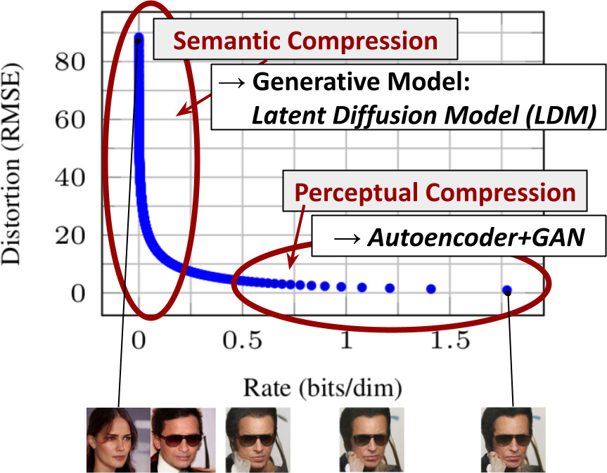
This two-stage approach provides the best of both worlds: the powerful inductive biases of the U-Net architecture are perfect for the spatially structured latent space, and the computational load is massively reduced because this space is so much smaller than the original pixel space.
Stable Diffusion from Scratch in PyTorch | Unconditional Latent Diffusion Models
Let's watch another segment from the 'ExplainingAI' video, which introduces this two-stage concept.
Watch the section from 04:19 to 05:27. It clearly explains the idea of training an autoencoder first and then running the diffusion process in its latent space.
3. The Quality Trade-Off: Building a High-Fidelity Autoencoder
The effectiveness of this entire approach hinges on the quality of the autoencoder. If the compression stage is "lossy" and discards important visual information, no matter how good the subsequent diffusion model is, the final generated images will be of poor quality.
The Problem with Simple Reconstruction Loss
If you were to train the autoencoder with a simple pixel-wise L1 or L2 reconstruction loss, the resulting images would be blurry. This is because these losses average over local pixel differences and are not sensitive to the high-frequency details that constitute sharp textures and edges.
Stable Diffusion from Scratch in PyTorch | Unconditional Latent Diffusion Models
Let's continue with the 'ExplainingAI' video to understand why a simple loss function is insufficient.
Watch from 07:31 to 08:37. This section explains why L1/L2 loss leads to blurry reconstructions and motivates the need for more perceptually-aligned losses.
The Solution: Combining Perceptual and Adversarial Losses
To create a high-fidelity autoencoder, the LDM paper leverages techniques from the VQGAN paper. The autoencoder is trained with a combination of loss functions:
- Reconstruction Loss (L1/L2): A standard pixel-wise loss to ensure the overall structure and color are correct.
- Perceptual Loss (LPIPS): Instead of comparing pixels directly, this loss compares the feature maps of the input and reconstructed images extracted from a pre-trained network (like VGG). This ensures the images are perceptually similar, which aligns better with human judgment.
- Adversarial Loss: A patch-based discriminator is trained to distinguish between real images and the autoencoder's reconstructions. This forces the autoencoder (acting as a generator) to produce highly realistic outputs with sharp details to "fool" the discriminator.
The following video segments provide an excellent conceptual overview of these advanced loss functions.
Stable Diffusion from Scratch in PyTorch | Unconditional Latent Diffusion Models
Let's finish the key conceptual parts of the 'ExplainingAI' video.
First, watch from 08:37 to 13:21 to understand perceptual loss. Then, watch from 16:16 to 19:32 for an explanation of adversarial loss in this context. These two segments are key to understanding the 'quality' side of the trade-off.
For a deeper dive into the implementation of these losses, which may be interesting given your engineering background, the following resource provides a detailed code walkthrough. It's a bit long, so feel free to skim, but it shows exactly how these loss components (including a VAE-style KL divergence regularizer) come together in practice.
Stable Diffusion: High-Resolution Image Synthesis with Latent Diffusion Models | ML Coding Series
This video from Aleksa Gordić's 'The AI Epiphany' channel walks through the PyTorch code for training the LDM autoencoder.
Watch from 15:23 to 40:43 to see how the perceptual loss (LPIPS) and adversarial loss (using a PatchGAN discriminator) are instantiated and calculated. Then, the summary from 44:49 to 45:45 provides a great recap of why each loss component is necessary.
By combining these losses, the autoencoder learns to create a compact latent representation that faithfully preserves the important perceptual details of the original image.
4. Analyzing the Trade-Offs Empirically
We've established the theoretical motivation: latent diffusion should be more computationally efficient while maintaining quality. Now, let's look at the empirical evidence from the LDM paper that validates this.
The key parameter in this trade-off is the downsampling factor (f) of the autoencoder. A larger f means more compression, a smaller latent space, and faster computation, but it risks more information loss.
The authors of the LDM paper conducted experiments with various downsampling factors. The results clearly show a "sweet spot."
High-Resolution Image Synthesis With Latent Diffusion ...
Let's look at the experimental results in the LDM paper that directly analyze these trade-offs.
Read Section 4.1, 'On Perceptual Compression Tradeoffs'. Pay close attention to Figure 5, which shows training progress for different factors f. Then, examine Table 6, which directly compares the training/sampling throughput and final quality (FID score) of a pixel-based model (LDM-1) versus a latent model (LDM-4).
The key findings from these experiments are:
- Too little compression (
f= 1, 2) is inefficient. The model is essentially still a pixel-space DM, and training is slow. - Too much compression (
f= 32) leads to information loss in the autoencoder, limiting the final achievable image quality. The model trains fast but plateaus at a worse FID score. - The sweet spot (
f= 4, 8) strikes an optimal balance. These models are significantly faster to train and run inference on than their pixel-space counterparts, and they even achieve better final quality because the diffusion model can focus all its capacity on modeling the rich semantic information in the latent space.
The data from Table 6 is particularly telling: LDM-4 shows a 2.7x speed-up in training throughput over LDM-1 while also achieving a 1.6x improvement in FID score. This demonstrates that latent diffusion is not just a compromise for efficiency; it's a superior approach for high-resolution synthesis.
Test your understanding!
Imagine you are tasked with creating a latent diffusion model for generating highly-detailed 4K (3840x2160) architectural visualizations. A colleague suggests using a very aggressive downsampling factor of f=32 for the autoencoder to maximize computational savings. This would shrink the input from 3840x2160 to 120x68.
Based on the trade-offs we've discussed, what would be your primary concern with this approach, and what would you recommend instead?
Show answer
My primary concern would be irreversible information loss during the perceptual compression stage. Architectural visualizations contain fine-grained details (textures, lighting, sharp geometric lines) that are crucial for realism. An aggressive downsampling factor of f=32 is very likely to destroy this high-frequency information. Even a perfect diffusion model trained on these degraded latents would be unable to reconstruct the original details, leading to blurry or simplified outputs.
Recommendation: I would recommend starting with a more moderate downsampling factor, such as f=8 or f=4, as suggested by the LDM paper's experiments. This strikes a better balance between computational efficiency and preserving perceptual fidelity. We could train autoencoders with f=4, f=8, and f=16 and evaluate their reconstruction quality (using metrics like PSNR, SSIM, and LPIPS) on our architectural dataset. We would choose the highest factor that still provides high-fidelity reconstructions before committing to training the full diffusion model. This two-stage evaluation process minimizes wasted compute while ensuring the foundation of our generative model is solid.
Conclusion
In this lesson, we dissected the core motivation behind Latent Diffusion Models. You now understand the critical trade-offs between computational cost and image quality that make this approach so effective.
Key Takeaways:
- The Problem: Pixel-space diffusion models are computationally expensive for high-resolution images because they operate on massive inputs and waste capacity on imperceptible details.
- The Solution: Latent diffusion is a two-stage process. It first uses a high-fidelity autoencoder to compress images into a small latent space, then runs the diffusion process efficiently within that space.
- The Quality Component: To avoid quality degradation, the autoencoder must be trained with a combination of reconstruction, perceptual, and adversarial losses to ensure its reconstructions are sharp and realistic.
- The Trade-off: There is an optimal compression factor. Too little compression is inefficient, while too much destroys information. Experiments show that downsampling factors of 4 or 8 often provide the best balance of speed and quality.
Next Lesson Preview:
We've covered the "why" and "what" of the perceptual compression stage. In the next lesson, we will put this theory into practice. Our goal will be to train a Variational Autoencoder (VAE) with perceptual and adversarial losses for high-fidelity image compression. This will be a hands-on implementation of the first, and most critical, component of a Latent Diffusion Model.