Bounding Client Metrics with Markov and Chebyshev Inequalities

Welcome back, Detective. Our last investigation concluded with a decisive verdict: the statistical evidence, in the form of a large F-statistic, confirmed that the type of relationship arrangement at Elysian Moments has a significant impact on client satisfaction. We closed that part of the case file, proving that the dispute between Anya and Ben was rooted in a real, measurable phenomenon.

However, a new lead has just emerged from the studio's disorganized archives. While searching for more satisfaction data, you've uncovered a partially corrupted financial summary page. It contains aggregated data on client spending for add-on services, but the individual transaction records are lost. For some client groups, we only have an average spending figure; for others, we have an average and a standard deviation. We can't reconstruct the full picture, but we can't let this clue go to waste.

In this lesson, we will learn how to make powerful, evidence-backed statements even with such incomplete information. We will apply two fundamental tools from your probabilistic toolkit—the Markov and Chebyshev inequalities—to establish credible bounds on these client metrics. This will allow us to test claims and narrow down possibilities, even when the exact distribution of the data remains a mystery.

The First Clue: A Vague Claim and a Simple Average

Among the recovered data fragments is a single, tantalizing number: for clients in the "Muse" arrangement, the average spending on ancillary services (like extra photoshoots or custom lingerie designs) was $80.

Shortly after you uncover this, a rumor starts circulating, planted by a rival studio, that Elysian Moments relies on a few "whale" clients who spend exorbitant amounts, and that a large proportion of "Muse" clients actually spend over $400. With only the average, this is hard to disprove directly. Or is it?

This is a classic scenario for Markov's inequality. It's our broadest tool, requiring only two conditions:

The random variable must be non-negative (which spending is).
We must know its mean (which we do).

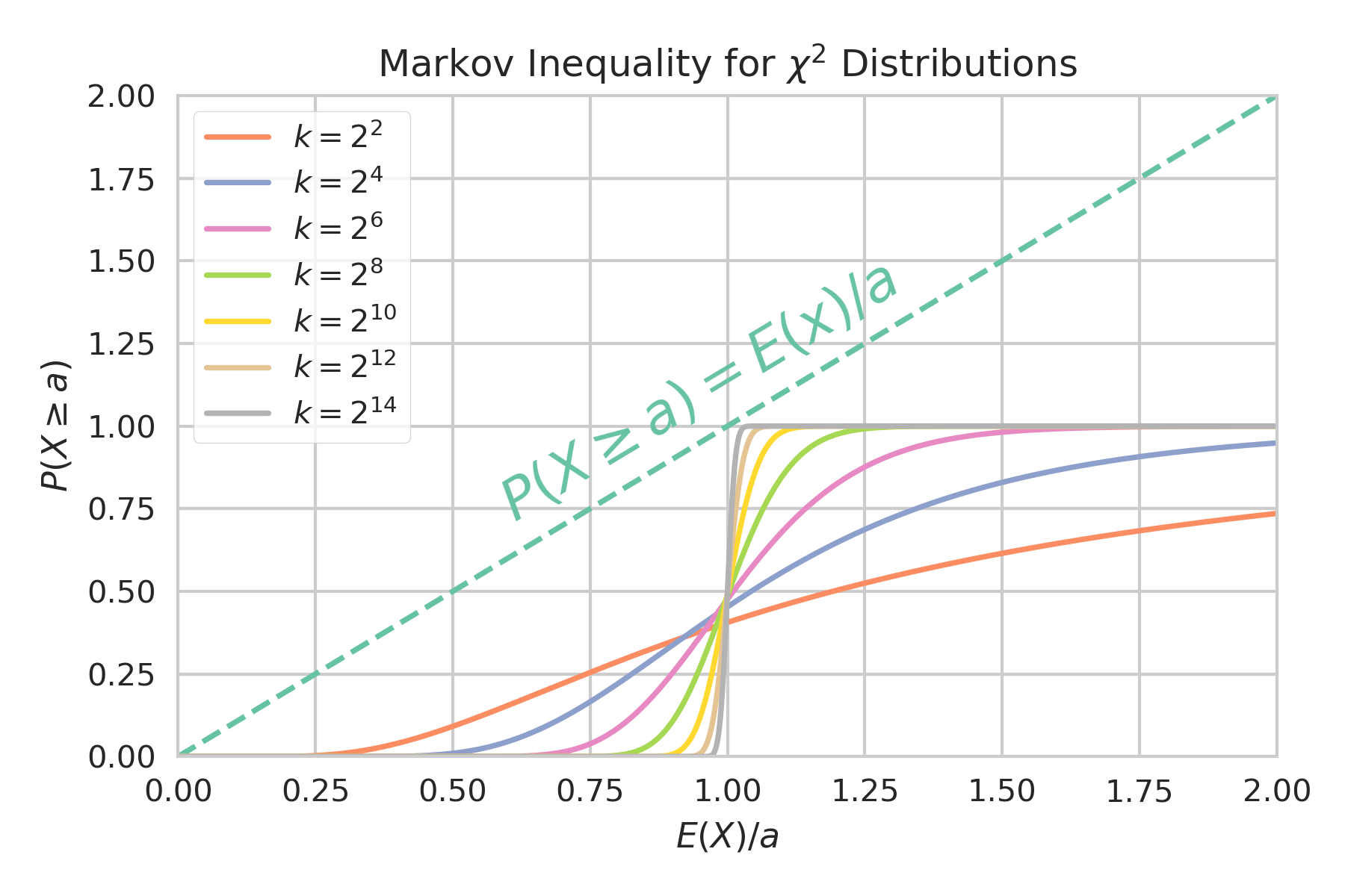
Markov's inequality provides a simple but powerful upper bound on the probability that a random variable will exceed some value.

Markov's Inequality

For a non-negative random variable $X$ with mean $E [X]$ , and for any value $a > 0$ , the inequality states:

P (X \geq a) \leq \frac{E [ X ]}{a}

The core intuition is that a distribution can't have too much mass placed far above the mean without pulling the mean itself up. The following video provides an excellent visual and conceptual walkthrough of this principle.

Markov's Inequality ... Made Easy!

This video, "Markov's Inequality ... Made Easy!" from the Stats with Brian channel, breaks down the inequality's logic with great intuition.

Watch the initial definition from the start. Then, focus on the section from the derivation, which uses the law of total expectation to build a strong intuition for why the bound must hold. Finally, watch the real-world example about income distribution, which is directly analogous to our client spending problem.

To formalize this, let's turn to a concise written resource.

6.1: Markov and Chebyshev Inequalities

This section from a set of Stanford course notes provides the formal definition and a clear proof.

Read the section titled "Markov's Inequality" for the setup. The exam score example that follows builds powerful intuition. Then, review the formal proof to solidify the concept.

Applying Markov's Inequality to the Case

Now, let's use this tool to investigate the rival studio's claim.

Let $X$ be the spending of a randomly chosen "Muse" client.
We know $X \geq 0$ .
We have the mean, $E [X] = $80$ .
The claim involves spending over $400, so we set our threshold $a = $400$ .

Applying Markov's inequality:

P (X \geq 400) \leq \frac{E [ X ]}{400} = \frac{80}{400} = \frac{1}{5} = 0.2

Our finding: At most, 20% of "Muse" clients could have spent $400 or more. While this doesn't completely refute the claim that some clients are "whales," it puts a firm, quantitative ceiling on how widespread this phenomenon can be. The rival's claim of a "large proportion" is now constrained by a hard number.

This graph illustrates the principle of Markov's inequality. The probability $P(X \ge a)$ for any non-negative distribution (the solid colored lines) must lie at or below the line $E(X)/a$ (the dashed line). Our calculation found the point on that dashed line that serves as the upper bound for our specific case.

The Second Clue: Adding Variance for a Sharper View

Encouraged, you manage to un-corrupt another fragment of the ledger. This one concerns the "Vixen" client group. For this group, you find not only the mean spending but also the standard deviation:

Mean spending ( $μ$ ): $150
Standard deviation ( $σ$ ): $30

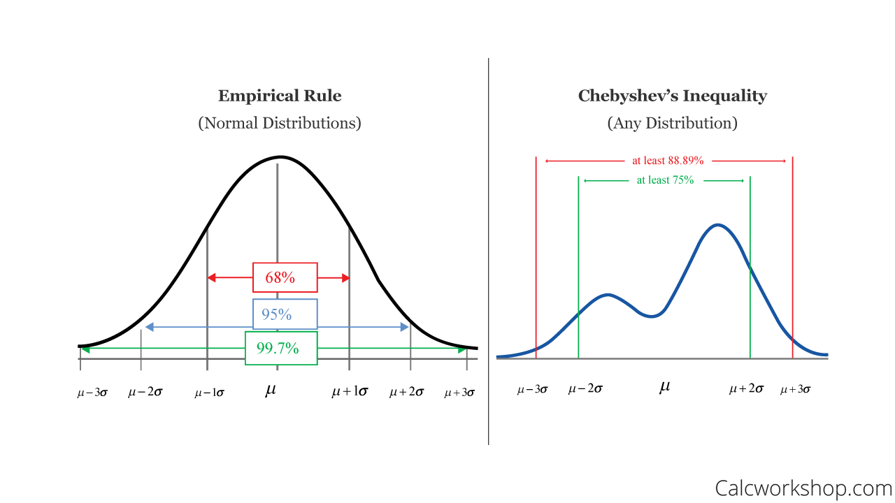
Now you have more information. This calls for a more powerful tool: Chebyshev's inequality. This inequality allows us to bound the probability that a random variable deviates from its mean by a certain amount, and it leverages variance to create a tighter bound.

Chebyshev's Inequality

For any random variable $Y$ with a finite mean $μ$ and variance $σ^{2}$ , and for any value $a > 0$ , Chebyshev's inequality states:

P (∣ Y - μ ∣ \geq a) \leq \frac{σ ^{2}}{a ^{2}}

Notice two key differences from Markov's:

It applies to any random variable, not just non-negative ones.
It bounds the probability of being in either tail (far above or far below the mean).

The proof is elegantly simple: it's just an application of Markov's inequality to the non-negative random variable $(Y - μ)^{2}$ .

Chebyshev's Inequality ... Made Easy!

The follow-up video, "Chebyshev's Inequality ... Made Easy!", clearly explains the concept and its relationship to Markov's inequality.

Watch the introduction from the beginning, which compares the two inequalities. Then, pay close attention to the step-by-step proof, which shows how Chebyshev's is a direct application of Markov's. Finally, the visual explanation provides another layer of intuition.

For a more formal treatment, including the direct proof, let's consult our lecture notes.

Lecture 3: Markov's, Chebyshev's, and Chernoff Bounds

These lecture notes from Rice University provide a concise, formal presentation of both inequalities.

First, briefly review the section on Markov's Inequality. Then, carefully study the subsequent section, "Chebyshev's Inequality". Note the proof, the corollary form P(|X - \mu| \ge k\sigma) \le 1/k^2, and the direct comparison between the two inequalities.

Applying Chebyshev's Inequality to the Case

Let's use this sharper tool on the "Vixen" client data. Suppose we want to determine the maximum possible proportion of clients whose spending is "extreme"—that is, more than $75 away from the mean of $150. This means their spending is either less than $75 ( $150 - 75$ ) or more than $225 ( $150 + 75$ ).

Let $Y$ be the spending of a randomly chosen "Vixen" client.
We have the mean, $μ = $150$ .
We have the variance, $σ^{2} = 3 0^{2} = 900$ .
We are interested in deviations of at least $75, so our threshold is $a = $75$ .

Applying Chebyshev's inequality:

P (∣ Y - 150∣ \geq 75) \leq \frac{σ ^{2}}{a ^{2}} = \frac{900}{7 5 ^{2}} = \frac{900}{5625} = 0.16

Our finding: There is, at most, a 16% chance that a "Vixen" client spends either less than $75 or more than $225. By incorporating the variance, we've created a more precise probabilistic boundary on the "tails" of the distribution.

This image perfectly summarizes our situation. If we knew the spending followed a Normal Distribution (left), we could use the Empirical Rule to say that 95% of data lies within 2 standard deviations. Since we don't know the distribution's shape, we must use Chebyshev's Inequality (right), which gives a more conservative but universally true bound: for any distribution, at least 75% of data lies within 2 standard deviations ($1 - 1/k^2 = 1 - 1/2^2 = 0.75$). Our inequalities are the tools for the detective who must work with unknown distributions.

Conclusion

In today's investigation, we've seen how to extract meaningful intelligence from seemingly sparse data. When faced with an unknown distribution and only summary statistics, we are not powerless. We can establish firm, provable bounds on the probabilities of certain outcomes.

Here are the key takeaways for your case file:

Markov's Inequality is your tool when you only have the mean of a non-negative variable. It provides a simple, one-sided bound: $P (X \geq a) \leq E [X] / a$ .
Chebyshev's Inequality is a more powerful tool for when you have both the mean and variance. It provides a tighter, two-sided bound on deviations from the mean for any distribution: $P (∣ X - μ ∣ \geq a) \leq σ^{2} / a^{2}$ .
The fundamental principle is that the more information you have about a distribution (from just a mean to a mean and variance), the more precise your probabilistic statements can be.

Preview of the Next Lesson

Our work on the ledger has uncovered yet another cryptic entry. It's a note from a previous analyst about "client engagement hours." Instead of reporting the average hours, the note reports the average of the logarithm of the hours. This seems odd. Why would someone transform the data before averaging it? What does $E [lo g (X)]$ tell us, and how does it relate to $lo g (E [X])$ ? In our next session, we'll delve into Jensen's inequality, a concept that governs the relationship between the expectation of a function of a random variable and the function of its expectation. This will reveal another layer of statistical subtlety and may uncover why the data was being presented in such a peculiar way.

Recommended resources