Bounding Expected Engagement with Jensen's Inequality

The Flaw of Averages

Before diving into the mathematics, let's build some intuition. We often assume that if we know the average of some input, we can just plug that average into a formula to get the average of the output. As you might suspect, reality is more complex. When the formula, or function, is non-linear, this intuition breaks down. This is often called the "flaw of averages."

The following video provides an excellent introduction to this concept, showing why 'average in' does not always lead to 'average out'.

As the video demonstrated, the relationship between $E[f(X)]$ and $f(E[X])$ depends entirely on the "shape" of the function $f$. This is where the concepts of convexity and concavity become our primary clues.

• A convex function is "bowl-shaped" upwards, like $f(x)=x^2$. A line segment connecting any two points on its graph lies above the function.
• A concave function is "bowl-shaped" downwards, like $f(x)=\log (x)$ or $f(x)=\sqrt{x}$. A line segment connecting any two points on its graph lies below the function.

Jensen's inequality formalizes this relationship:

For a random variable $X$ and a function $\phi$:

1. If $\phi$ is convex, then $\phi (E[X])\le E[\phi (X)]$.
2. If $\phi$ is concave, then $\phi (E[X])\ge E[\phi (X)]$.

The function of the average is always "pulled" towards the flatter part of the curve, while the average of the function accounts for the more extreme values produced by the function's curvature.

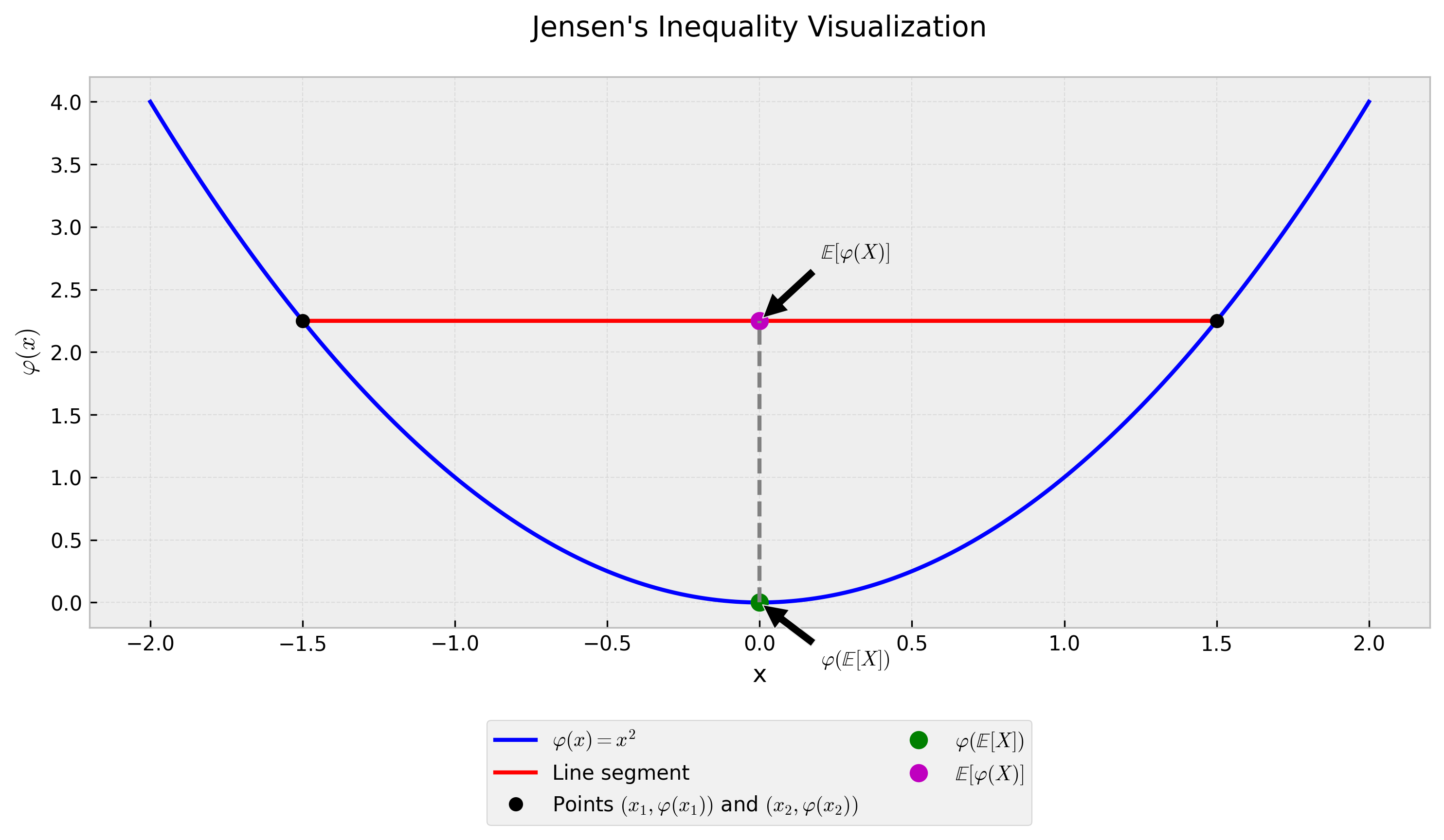
To solidify this concept, the next video offers a crisp, elegant visual walkthrough of the inequality and its proof.

Given your background, you may also appreciate a more formal, analytical proof. The following reading uses a Taylor series expansion to prove the inequality, a common technique in mathematical statistics.

Cracking the Analyst's Code

Now, let's apply this to the case. The cryptic note concerns the "Enigma" client group and reads: "Average of log-engagement-hours: 3.5". The studio management, unaware of the "flaw of averages," has interpreted this to mean the average engagement is simply $\exp (3.5)\approx 33.1$ hours. They are preparing a report based on this number. Let's verify their conclusion.

1. The Random Variable: Let $X$ be the engagement hours of a randomly selected "Enigma" client.
2. The Clue: We are given $E[\log (X)]=3.5$.
3. The Function: The transformation is $\phi (x)=\log (x)$.
4. The Function's Shape: The natural logarithm function is concave.
5. Applying the Tool: For a concave function, Jensen's inequality states: $$\log (E[X])\ge E[\log (X)]$$
6. Substituting and Solving: We substitute the value from the note: $$\log (E[X])\ge 3.5$$ To solve for $E[X]$, we exponentiate both sides: $$E[X]\ge e^{3.5}\approx 33.12$$

The Revelation: The management's assumption is wrong. The true average engagement, $E[X]$, is not equal to 33.1 hours, but is greater than or equal to 33.1 hours. The value reported by the analyst provides a lower bound for the true average engagement. This is a subtle but critical distinction. The analyst wasn't trying to hide a low number; their note, when correctly interpreted, actually suggests the average engagement is at least 33.1 hours.

This specific application of Jensen's inequality with the log function is famously used to prove the inequality of arithmetic and geometric means (AM-GM). The following reading explores this exact scenario.

A Second Clue: The Bonus Payout Puzzle

Let's test our understanding on another fragment of data. For the "Shadow" client group, we have a simple average: their mean engagement is 20 hours. A new incentive program promises a bonus payout to consultants proportional to the square of their client engagement hours. A manager has estimated the average bonus payout by simply squaring the average engagement: $20^2=400$. Is this estimate accurate, or is it an over- or underestimate?

1. The Random Variable: $X$ = engagement hours, with $E[X]=20$.
2. The Function: The bonus is tied to $\phi (x)=x^2$.
3. The Function's Shape: The square function is convex.
4. Applying the Tool: For a convex function, Jensen's inequality states: $$(E[X]{)}^2\le E[X^2]$$
5. Substituting: $$20^2\le E[X^2]$$ $$400\le E[X^2]$$

The Revelation: The manager's estimate of 400 is an underestimate. The true average bonus payout, $E[X^2]$, is guaranteed to be greater than or equal to 400. The gap between $E[X^2]$ and $(E[X]{)}^2$ is, in fact, the variance of $X$. The manager's simple calculation completely ignored the impact of variability in engagement hours, which will always push the average of the squared values higher.

Conclusion

Our investigation today has added a powerful and subtle tool to your arsenal. By understanding Jensen's inequality, we can now correctly interpret summary statistics that involve non-linear transformations and establish rigorous bounds on unknown quantities. This moves us beyond simple averages into a more nuanced understanding of how distributions behave under transformation.

Here are the key takeaways for your case file:

• The "Flaw of Averages": For a non-linear function $\phi$, plugging in the average input, $\phi (E[X])$, does not give you the average output, $E[\phi (X)]$.
• Jensen's Inequality provides the correction. The direction of the inequality depends on the function's shape:
  • For convex functions ($x^2$, etc.): $\phi (E[X])\le E[\phi (X)]$. The function of the average provides a lower bound on the average of the function.
  • For concave functions ($\log (x)$, $\sqrt{x}$, etc.): $\phi (E[X])\ge E[\phi (X)]$. The function of the average provides an upper bound on the average of the function.
• This principle allows a detective to spot misleading claims and derive bounds from transformed data, turning a potentially confusing clue into a piece of hard evidence.

Preview of the Next Lesson

We have now concluded our analysis of the static data in the "Arrangement Dispute" case file. From satisfaction scores to spending and engagement metrics, we have squeezed every drop of insight from these summary statistics.

But many of the mysteries at Elysian Moments unfold over time. In our next module, "The Booking Pattern Conspiracy," we will shift our focus from static snapshots to dynamic processes. We will begin by learning how to model the arrival of events—such as photoshoot booking requests—over time. This will allow us to ask crucial new questions: Is a sudden flurry of bookings a sign of success, or something more suspicious? Is a long silence between clients normal, or a signal of trouble? Our investigation is about to enter the dimension of time.