Welcome back, Detective. In our last session, we took the initial, crucial step in untangling "The Arrangement Dispute" at Elysian Moments. We meticulously partitioned the total variation in client satisfaction scores (SST = 38) into two key components: the variation between the different relationship arrangements (SSB = 32) and the random variation within those arrangements (SSW = 6).
Our preliminary finding was a strong clue: the variation attributable to the arrangement type seems to vastly outweigh the background noise. Today, we elevate this clue into hard evidence. We will formalize our analysis by computing the F-statistic, a definitive measure that will allow us to formally assess whether the satisfaction differences are statistically significant or merely a product of chance.
From Raw Sums to Fair Averages: Mean Squares
Before we can calculate our final test statistic, we need to account for the fact that the Sums of Squares we calculated (SSB and SSW) are influenced by the amount of data we have. To create a standardized, fair comparison, we must convert these sums into averages, or what are known in statistics as Mean Squares (MS).
However, we don't just divide by the number of data points. In statistics, the proper divisor is the degrees of freedom (df), which, as you know from your background in experimental design, represents the number of independent pieces of information used to calculate the statistic.
For our case, the degrees of freedom are:
- Degrees of Freedom Between Groups (): This is the number of groups () minus one.
- Degrees of Freedom Within Groups (): This is the total number of observations () minus the number of groups ().
Now we can calculate the Mean Squares:
- Mean Square Between (MSB): This is the average variation between the groups. It represents the "signal" we are trying to detect.
- Mean Square Within (MSW): This is the average variation within the groups, often considered the "error" or "noise" term.
The following resource provides a clear walkthrough of these calculations, which confirms the steps we've just taken.
Chapter 16: One-Way ANOVA Tests
This chapter details the manual calculation process for an ANOVA test. It's a useful reference to formalize our procedure.
Focus on the section describing the calculation of Mean Squares. You can find this by searching for the formulas for MSB and MSW. Specifically, review the two equations. Notice how they align perfectly with the calculations we just performed.
The F-Statistic: Quantifying the Signal-to-Noise Ratio
With the Mean Squares calculated, we can now compute the centerpiece of our analysis: the F-statistic. This statistic is simply the ratio of the two mean squares we just found.
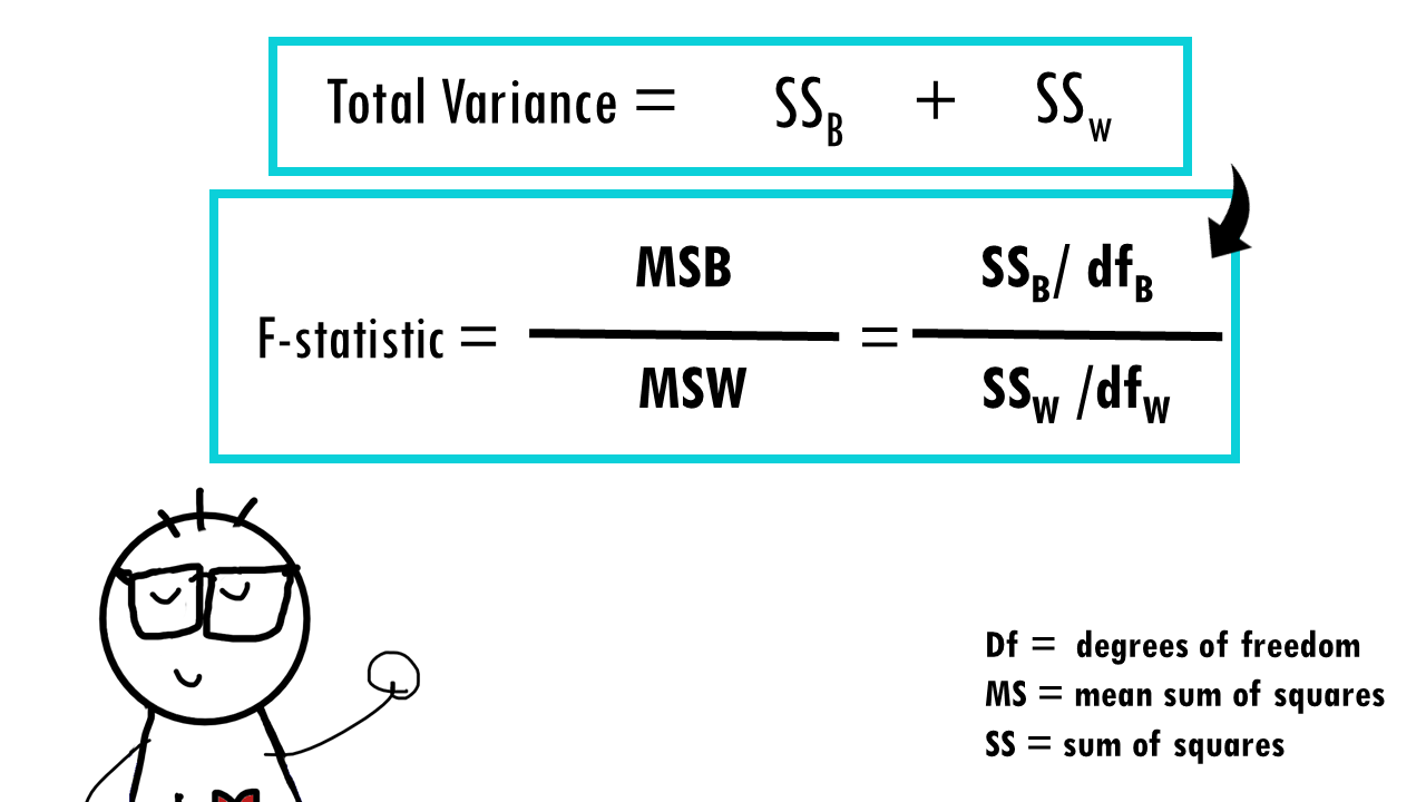
The F-statistic provides a single number that captures the signal-to-noise ratio in our data. A large F-value suggests that the variation between groups (the signal) is much larger than the variation within groups (the noise), indicating a real effect. An F-value close to 1 suggests the signal is indistinguishable from the noise.
For the Elysian Moments case, the F-statistic is:
An F-value of approximately 24 is quite large. It tells us that the observed variation between the satisfaction scores of the different arrangement types is about 24 times larger than the random variation within those types. This is a very strong piece of evidence.
To deepen your intuition about what this ratio represents, the following article by Jim Frost provides an excellent conceptual breakdown.
How F-tests work in Analysis of Variance (ANOVA)
This article eloquently explains the logic behind the F-test, focusing on the meaning of its numerator and denominator.
Read through the article starting from the section "The F-test in One-Way ANOVA". Pay close attention to the conceptual explanations of the numerator (our "signal") and the denominator (our "noise"). Finally, examine the section on the F-statistic itself, which uses helpful graphics to show how different combinations of signal and noise lead to different F-values.
For a quick visual summary of these concepts, the following video from Stats with Brian is also quite effective.
Analysis of Variance (ANOVA) and F statistics .... MADE EASY!!!
This video provides an animated, intuitive explanation of the core concepts behind the F-statistic.
Watch the segment explaining between-group and within-group variance. Then, focus on the definition and interpretation of the F-statistic as the ratio of these two variances.
The Verdict: Reaching a Statistical Conclusion
We have a suspect (the arrangement type), a motive (it appears to cause different satisfaction levels), and a powerful piece of evidence (an F-value of 24). Now, we must present our case in the formal language of hypothesis testing.
- The Null Hypothesis (): The court of chance assumes innocence. It posits that there is no real difference in mean satisfaction scores among the three arrangement types (). The variations we see are purely random.
- The Alternative Hypothesis (): Our claim as detectives. We argue that at least one arrangement type has a different mean satisfaction score from the others.
To decide between these, we ask: "How likely is it that we would get an F-value as large as 24 if the null hypothesis were true?"
To answer this, we compare our F-value to the F-distribution, which is the theoretical probability distribution of F-values under the assumption that is true. The specific shape of this distribution is defined by our two degrees of freedom: and .
For an F-distribution with (2, 9) degrees of freedom, the critical value for a standard significance level of is 4.26.
- Our calculated F-value: 23.99
- The critical F-value: 4.26
Since our calculated F-value is far greater than the critical value, it falls deep into the "rejection region." This means our result is extremely unlikely to have occurred by chance. The probability of observing an F-value of 23.99 or higher, if there were truly no difference between the groups, is exceedingly small (p < 0.001).
Therefore, we reject the null hypothesis. The evidence is statistically significant. We can confidently report to the owner of Elysian Moments that the dispute between Anya and Ben is not based on anecdotal evidence or random noise. The type of relationship arrangement has a demonstrable and significant impact on client satisfaction.
Assembling the Case File: The ANOVA Table
The standard way to present the findings of an ANOVA is in a summary table. This neatly organizes all the evidence we've gathered and calculated.

Here is the completed ANOVA table for "The Arrangement Dispute":
| Source | Degrees of Freedom (df) | Sum of Squares (SS) | Mean Squares (MS) | F-statistic | P-value |
|---|---|---|---|---|---|
| Between Groups | 2 | 32 | 16 | 23.99 | < 0.001 |
| Within Groups (Error) | 9 | 6 | 0.667 | ||
| Total | 11 | 38 |
This table serves as the final, conclusive report of our statistical investigation.
Conclusion
Today, we have moved from preliminary clues to a definitive statistical verdict. By converting our Sums of Squares into Mean Squares and calculating the F-statistic, we quantified the signal-to-noise ratio in the Elysian Moments satisfaction data. Comparing our high F-value to its corresponding F-distribution allowed us to formally reject the null hypothesis.
The key takeaways from this investigation are:
- The F-statistic is calculated as the ratio of Mean Square Between (MSB) to Mean Square Within (MSW).
- MSB and MSW are found by dividing the Sum of Squares (SSB and SSW) by their respective degrees of freedom ( and ).
- The F-statistic represents a "signal-to-noise" ratio, where a larger value indicates a stronger effect.
- By comparing our calculated F-value to a critical value (or by examining its p-value), we can determine if the observed differences between group means are statistically significant.
- For the Elysian Moments case, the evidence is conclusive: the relationship arrangement type has a significant effect on client satisfaction.
Preview of the Next Lesson
While we have settled the primary dispute, this case is not closed. In the process of reviewing the studio's records, a new piece of evidence has surfaced: a partially redacted financial ledger showing client spending on ancillary services. The data is incomplete, with only means and variances available for some groups. In our next session, we will turn our analytical toolkit to this new problem. We will employ powerful probabilistic bounds—specifically the Markov and Chebyshev inequalities—to determine what we can deduce from this limited information, opening a new and potentially more revealing line of inquiry into the studio's operations.