Predicting Customer Churn with Logistic Regression

Welcome back, Detective.

The ink is barely dry on our final report for the "Fixed Survey" case, where we uncovered a sophisticated data forgery at Elysian Partners. Our investigation revealed a dataset so perfectly crafted, so devoid of real-world noise, that its very perfection was the ultimate confession. We proved that their entire client satisfaction database was likely generated from a formula, not from people.

A new case file has just arrived, presenting a challenge of a different nature. The owner of "Velvet Veil," an exclusive boudoir photography studio, is facing a perplexing issue: a high rate of client attrition. Many clients have a wonderful first session but then vanish, never returning for follow-up shoots or to purchase premium photo albums. They aren't complaining; they're simply disappearing. The owner wants to know why, and more importantly, who is likely to disappear next.

Our previous tool, multiple linear regression, was designed to predict a continuous value—a satisfaction score on a scale. Here, the outcome isn't a score; it's a binary event. A client either returns (let's call that '1') or they don't ('0'). We need a different tool from our kit, one capable of handling a "Yes/No" mystery. This investigation will require us to model not a specific value, but the probability of an event occurring.

Clue #1: The Limits of a Straight Line

In our last case, we modeled client satisfaction with a linear equation. It worked because we were predicting a number that could, in theory, go up or down indefinitely. But what happens if we try to apply that same logic here? Our outcome can only be 0 or 1.

Imagine we plot our client data, with some predictor like "Initial Spending" on the x-axis and the outcome "Returned" (0 or 1) on the y-axis. A linear regression model would try to fit a straight line through these points.

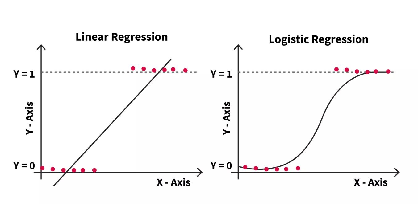
A comparison of fitting a linear regression model (left) versus a logistic regression model (right) to data with a binary outcome (Y=0 or Y=1).

Look at the "Linear Regression" plot on the left. The line extends beyond 1 and below 0. What would a predicted value of 1.3 mean? A 130% chance of returning? Or -0.2, a -20% chance? These values are nonsensical. A straight line is the wrong shape for this kind of problem.

The plot on theright, "Logistic Regression," suggests a more elegant solution: an S-shaped curve, known as a sigmoid curve. This curve is perfectly constrained between 0 and 1, making it ideal for modeling probabilities. Our task is to find a model that produces such a curve.

Clue #2: The Probability Lens

The core of our new technique is to shift our thinking. Instead of predicting the outcome (0 or 1) directly, we will predict the probability of the outcome being 1. For this, we'll use a method that connects a linear model to a probability model.

The Medium article "Customer Churn Data Analysis using Logistic Regression" provides an excellent high-level overview of this exact problem, just in a different industry.

Customer Churn Data Analysis using Logistic Regression

This article frames the problem of predicting customer churn, which is analogous to our "disappearing client" problem. It sets the stage for why we need a specialized classification model.

Read the introduction and the sections titled "Role of Data Analytics" and "What will we do?". Focus on how the author frames the problem as a binary classification task—predicting a "Yes" or "No" output.

The tool we need is logistic regression. It's a member of the generalized linear model family, which you'll know from your econometrics and DoE background. The genius of this method is that it uses the familiar linear equation $(β_{0} + β_{1} X_{1} + \dots)$ but transforms its output to produce the S-shaped probability curve we need.

This transformation happens in two steps:

The model predicts the log-odds of the event, which can range from $- \infty$ to $+ \infty$ , just like a linear regression output.
This log-odds value is then converted into a probability (a number between 0 and 1) using the inverse logit or logistic function.

The online textbook chapter "Logistic Regression" explains this transformation formally. Given your statistical training, you'll find the mathematical foundation here quite direct.

Chapter 8 Logistic Regression

This chapter explains the mathematical bridge between a standard linear model and the probability model used in logistic regression.

Read the introduction to understand the role of the logit function, which transforms probability into log-odds: Logit Function. Then, read the next section, "The inverse logit function," to see how we reverse this process to get from the model's output back to a meaningful probability. This function is the S-shaped curve we're looking for.

The logistic regression equation, which implements this inverse logit function, looks like this:

P (Y = 1∣ X) = \frac{1}{1 + e ^{- (β_{0} + β_{1} X_{1} + \dots + β_{n} X_{n})}} = \frac{e ^{(β_{0} + β_{1} X_{1} + \dots + β_{n} X_{n})}}{1 + e ^{(β_{0} + β_{1} X_{1} + \dots + β_{n} X_{n})}}

The term in the exponent is simply the linear regression equation we already know. This entire expression is the sigmoid function that squashes the linear output into the [0, 1] range.

Clue #3: Preparing the Evidence

Before we can build our model, we must prepare the client data from Velvet Veil studio. Just like in our previous cases, this involves some crucial preprocessing steps. The model also rests on a few key assumptions.

Customer Churn Data Analysis using Logistic Regression

This part of the article outlines the practical steps of data preparation and the key assumptions you must check before fitting a logistic regression model.

First, read the section on Assumptions. Pay attention to the need for an independent, binary dependent variable and the absence of multicollinearity. Next, read about Data Preparation. The creation of dummy variables for categorical data (like Package_Type) and normalization of continuous data (like Age or Initial_Spending) are critical forensic steps.

With our data prepared, we are ready to fit the model. This is typically done with statistical software using a function like glm() (generalized linear model) with the family argument set to binomial, which specifies that we are modeling a binary outcome.

Clue #4: Building the Model and Making a Prediction

Fitting the model will give us the coefficient estimates ( $β$ 's) for each predictor in our case file. As we learned, these coefficients are in log-odds units, which aren't intuitive. The final and most crucial step is to use these coefficients to predict the probability of a client returning.

The "Logistic Regression" chapter demonstrates exactly how to do this.

Chapter 8 Logistic Regression

This reading shows you how to fit the model and, most importantly, how to use the fitted model to calculate the probability for a new observation.

First, look at the section "Logistic regression example" to see how a model is fitted in R. Notice the use of glm() with family = binomial. Next, read the section on interpreting coefficients. This is the core of our task: it shows how to plug coefficients and variable values into the inverse logit function to get a probability. Note the crucial point that the effect of a predictor is non-linear—its impact on probability depends on the values of the other predictors. Finally, review the section "Using the model to predict probabilities." This shows the full process of creating a new data profile and using the predict() function to generate a probability, which is exactly what our learning outcome requires.

Let's put this into practice. Suppose our analysis of the Velvet Veil data yields the following model:

log-odds (Return) = - 2.0 + 1.2 \times EngagementScore - 0.8 \times BookedViaDiscount + 0.04 \times Age

Here, EngagementScore is a metric from 0-5, BookedViaDiscount is a dummy variable (1 if true, 0 if false), and Age is the client's age in years.

Now, let's profile a new client: a 35-year-old who booked without a discount (BookedViaDiscount = 0) and had an EngagementScore of 3.

Calculate the linear component (log-odds):
$log-odds = - 2.0 + (1.2 \times 3) - (0.8 \times 0) + (0.04 \times 35)$ $log-odds = - 2.0 + 3.6 - 0 + 1.4 = 3.0$
Convert log-odds to probability:
$P (Return) = \frac{1}{1 + e ^{- 3.0}} \approx \frac{1}{1 + 0.0498} \approx 0.952$

Our model predicts this client has approximately a 95% probability of returning. This is the kind of actionable intelligence the studio owner needs.

Conclusion of the Initial Investigation

In this session, we've added a powerful new instrument to our detective toolkit. We established that for binary ("Yes/No") outcomes, linear regression is unsuitable, as it can produce nonsensical predictions. We then constructed our first logistic regression model, a method that uses a linear combination of predictors to model the log-odds of an event and then transforms this output into an interpretable probability using the sigmoid (inverse logit) function. By building this model for Velvet Veil studio, we can now take any client's profile and calculate the precise probability that they will become a "disappearing client."

Preview of the Next Case

Our current model helps predict individual client behavior. However, the studio owner has another suspicion. They offer three distinct "relationship arrangement" packages: one for individuals in monogamous relationships, one for those in open relationships, and a more elaborate one for polyamorous groups. The owner feels that satisfaction seems to differ across these groups but has no hard evidence.

To investigate this, we'll need a method specifically designed to compare the average satisfaction scores across multiple, distinct groups. This will lead us into our next case, "The Arrangement Dispute," where we will use a tool to analyze variance and determine if the type of relationship arrangement truly has a statistically significant impact on client satisfaction.