Welcome back, Detective.
In our last briefing, we identified our primary tool for the "Disappearing Clients" case: logistic regression. We established how to take the profile data from Velvet Veil studio and construct a model that calculates the probability of a client returning. We've already run a calculation for one specific client, but a single data point doesn't solve a case. Now, we must put the entire model on the stand and interrogate it. Is it a reliable witness, or is it just telling us what we want to hear? How well does it actually explain the pattern of client attrition we're seeing?
This lesson is about model evaluation. We need to move beyond predicting for one person and assess the model's overall performance. This is the crucial step that separates a flimsy theory from hard evidence. We will approach this systematically, examining the model from several angles to build a complete picture of its strengths and weaknesses.
Angle 1: Is the Model Telling Us Anything at All?
Before we trust any specific prediction, we need to answer a fundamental question: Is our model, with all its client data, any better than a random guess? Our baseline "model of ignorance" would be to simply use the overall rate of attrition. If 40% of clients disappear, our null hypothesis is that every client has a 40% chance of disappearing, regardless of their profile. Our logistic regression model claims it can do better by using predictors like EngagementScore and Age.
The test for this is a likelihood-ratio chi-square test. It formally compares the log-likelihood of our fitted model to the log-likelihood of the "null" model (the one with only an intercept, representing the overall probability). A significant p-value tells us that our model's predictors, taken together, provide a statistically significant improvement over simply using the average.
The StatQuest video "Logistic Regression Details Pt 3: R-squared and p-value" offers an excellent visual walkthrough of this concept.
Logistic Regression Details Pt 3: R-squared and p-value
Josh Starmer explains how to derive a p-value for the overall model by comparing the log-likelihoods of the fitted and null models.
Watch the final section on calculating the p-value, p-value calculation. Focus on how two times the difference in log-likelihoods follows a chi-squared distribution, which gives us the p-value for the model as a whole.
This test is our first piece of evidence. If the p-value is low (e.g., < 0.05), we can reject the null hypothesis and conclude our model has explanatory power. We have grounds to proceed with the investigation.
Angle 2: How Much Does It Explain?
Knowing the model is significant is one thing; knowing how significant is another. This is where we look for an equivalent to the from linear regression. In OLS, is the "proportion of variance explained." For logistic regression, it's not so simple, leading to a family of what are called pseudo R-squared measures. They all aim to quantify the model's predictive power on a scale from 0 to 1.
The StatQuest video also provides the best intuitive foundation for this. It draws a direct analogy from the Sum of Squares in linear regression to the Log-Likelihood in logistic regression.
Logistic Regression Details Pt 3: R-squared and p-value
This part of the video explains why we can't use the standard R-squared and how log-likelihood can be used as an effective substitute to create a similar metric.
First, watch the quick review of how R-squared works in linear regression. Then, see how this concept is adapted for logistic regression using log-likelihoods for a "good fit" and a "bad fit" in this section. Finally, watch the demonstration that this new R-squared behaves as expected, going from 0 for a useless model to 1 for a perfect model.
While the principle is sound, there's no single, universally agreed-upon formula. The blog post "What's the Best R-Squared for Logistic Regression?" by statistician Paul Allison provides an excellent field guide to the most common suspects.
What's the Best R-Squared for Logistic Regression?
This post clearly explains the rationale and calculation for several popular pseudo R-squared measures, and makes a strong case for one in particular due to its intuitive appeal.
Read through the post to understand the three main candidates: McFadden’s R², which is interpreted as a proportional reduction in the model's "error." Cox & Snell's R², which has a strong theoretical link to OLS R² but suffers from an upper bound that can be much less than 1. Tjur’s R². This is perhaps the most intuitive for our detective work. It's simply the difference between the average predicted probability for clients who did return and the average predicted probability for those who disappeared. A large difference means the model is doing a good job separating the two groups.
For our case, Tjur's offers a very practical measure of our model's ability to distinguish between a loyal client and a "disappearing" one. A value of 0.25, for instance, would mean there is a 25-point difference in the average predicted probability of returning between the two actual groups.
Angle 3: How Good Are Its Predictions in Practice?
Now we get to the most practical test. If we use our model to label clients as either "likely to return" or "likely to disappear," how often are we right?
This requires setting a classification threshold. Typically, this is 0.5. If the model predicts a probability > 0.5, we classify the client as "returning"; if ≤ 0.5, we classify them as "disappearing." We can then create a confusion matrix, a tool you're already familiar with from your work on Bayesian inference and classifier performance.
The numiqo video "Logistic Regression [Simply explained]" gives a straightforward example of reading one of these tables.
Logistic Regression [Simply explained]
This short clip shows how to interpret a classification table, which is identical in principle to a confusion matrix.
Watch the section from the results table to the end of the classification table explanation. This will show you how to calculate the model's overall accuracy.
While accuracy is useful, the choice of 0.5 as a threshold is arbitrary. For Velvet Veil studio, it might be more important to correctly identify clients who are likely to disappear (high sensitivity) even if it means wrongly flagging some who would have returned (lower specificity). To evaluate the model across all possible thresholds, we use the Receiver Operating Characteristic (ROC) curve.
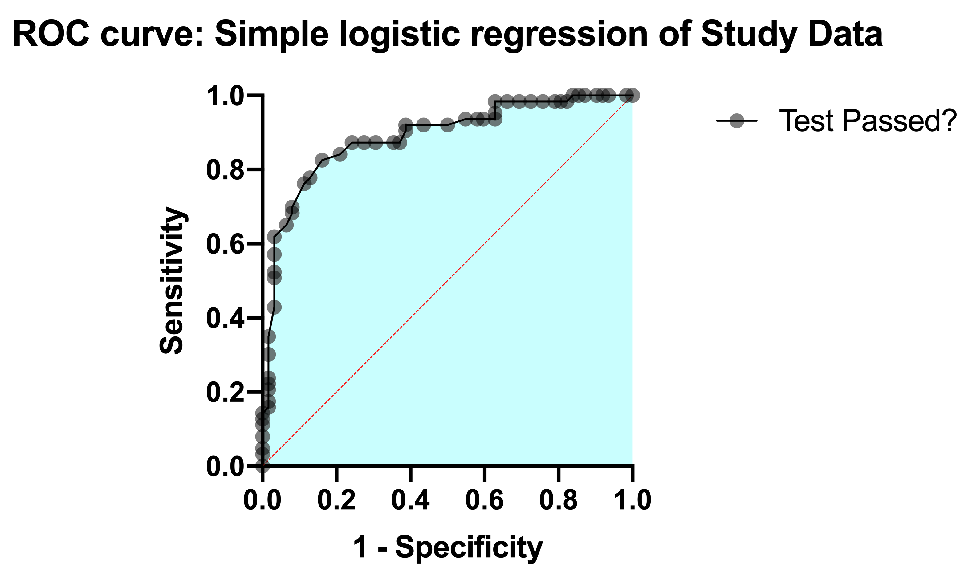
The ROC curve visualizes the trade-off. The diagonal line represents a model with no predictive power (random chance). The more the curve pulls toward the top-left corner, the better the model is at separating the two classes.
We can summarize this entire curve with a single number: the Area Under the Curve (AUC).
- AUC = 1.0: A perfect classifier.
- AUC = 0.5: A useless classifier, equivalent to a coin flip.
- AUC > 0.7: Generally considered an acceptable model.
- AUC > 0.8: Considered a good model.
- AUC > 0.9: Considered an excellent model.
The AUC gives us a robust, threshold-independent measure of our model's classification ability.
Angle 4: Is the Model's Form Correct?
This final angle is more subtle, but critical given your statistical expertise. We've assessed the model's predictive power, but is the model correctly specified? A goodness-of-fit (GOF) test addresses this. It tests the null hypothesis that the fitted model is correct, meaning we don't need to add complexity like non-linear terms (e.g., Age squared) or interactions (e.g., Age * EngagementScore).
The most common GOF test is the Hosmer-Lemeshow (HL) test, but it has serious flaws. A more robust investigation requires knowing these limitations and the alternatives. The paper "Measures of Fit for Logistic Regression" is the definitive guide.
[PDF] Measures of Fit for Logistic Regression | Statistical Horizons
This paper explains the difference between measuring predictive power and testing for goodness-of-fit, details the problems with the standard HL test, and proposes more reliable alternatives.
Please read the following sections: The Introduction, to understand the crucial distinction between predictive power (R-squared) and what GOF tests are actually testing. The section detailing the problems with the Hosmer-Lemeshow test. This is key to understanding why we should be skeptical of it. The introduction to new GOF tests. You don't need to master the formulas, but understand the names and purposes of the alternatives, such as the Standardized Pearson test and the Stukel test, which are designed for the common situation where we have continuous predictors and ungrouped data.
A high p-value on a reliable GOF test gives us confidence that our model's linear, additive form is a reasonable representation of the underlying relationships. A low p-value would be a clue that we need to dig deeper and investigate more complex relationships between our variables.
Conclusion of the Evaluation
We have now subjected our model to a rigorous, multi-faceted interrogation. We didn't just ask if it worked; we asked how it worked. We've learned to:
- Test for overall significance using the chi-square test.
- Quantify its explanatory power using pseudo R-squared measures like Tjur's R².
- Evaluate its real-world classification performance using a confusion matrix, ROC curve, and AUC.
- Assess the correctness of the model's form using goodness-of-fit tests, while being aware of the pitfalls of the common Hosmer-Lemeshow test.
By examining the evidence from all these angles, we can now confidently state whether the model we've built is a trustworthy tool for understanding client attrition at Velvet Veil.
Preview of the Next Stage of Investigation
Assuming our model has passed its interrogation, we have a reliable tool. But a tool is only useful if you know how to read its results. The model coefficients we have are in "log-odds" units, which are not intuitive. Our next task is to translate these cryptic numbers into something actionable for the studio owner. We will learn how to convert coefficients into odds ratios, allowing us to say exactly how a one-unit change in a predictor—like an increase in EngagementScore or Age—multiplies the odds of a client disappearing. This will finally allow us to pinpoint the master culprits behind the "Disappearing Clients."