Interpreting Coefficients as Odds Ratios for Client Disappearance

Welcome back, Detective.

In our last session, we put our logistic regression model on the stand. Through a series of rigorous tests—likelihood ratios, pseudo R-squareds, ROC curves—we confirmed its integrity. It is a reliable witness. We now know that the model we built to explain the pattern of disappearing clients at Velvet Veil studio has genuine predictive power.

But a reliable witness is only useful if you can understand their testimony. The model's coefficients are currently in the language of log-odds, a form of statistical shorthand that is precise but not intuitive. Our mission today is to crack this code. We will translate these coefficients into odds ratios, a language that speaks directly to risk and probability. This will allow us to move from simply predicting who might disappear to understanding why they disappear, finally pinpointing the key factors that drive clients away.

From Probabilities to a Linear World

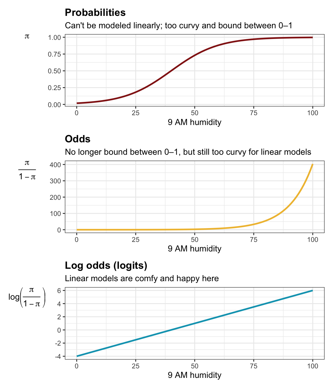
Before we can interpret the coefficients, let's briefly revisit the heart of logistic regression. We are trying to model a binary outcome (client returns vs. disappears), which is a probability, $π$ . The problem is that probabilities are bounded between 0 and 1, and their relationship with predictors is often non-linear and S-shaped. This makes them difficult to model directly with a linear equation.

The logistic model solves this by transforming the outcome. It doesn't model the probability $π$ itself, but rather the log-odds of the outcome, also known as the logit.

Probability ( $π$ ): The chance of an event happening. Ranges from 0 to 1.
Odds: The probability of the event happening divided by the probability of it not happening. Calculated as $\frac{π}{1 - π}$ . Ranges from 0 to $\infty$ .
Log-odds (Logit): The natural logarithm of the odds. Calculated as $lo g (\frac{π}{1 - π})$ . Ranges from $- \infty$ to $+ \infty$ .

This final transformation is the key. The log-odds can be modeled as a simple linear combination of our predictors, which is what our regression model does. The image below perfectly illustrates this journey.

These three plots show how we transform a bounded, S-shaped probability (top) into a simple, straight line (bottom) that a linear model can work with. Our model's coefficients live in the world of log-odds.

The foundational concepts of this transformation are explained well in a guide from the UCLA Statistical Consulting Group.

FAQ: How do I interpret odds ratios in logistic regression?

This document provides a clear, step-by-step explanation of the transformation from probability to log-odds, which is the foundation for our entire investigation.

Please read the first section, From probability to odds to log of odds. Focus on understanding how the range of the variable changes with each transformation and why this makes the log-odds suitable for linear modeling.

Our model's coefficients, like $β_{1}$ in the equation $logit (p) = β_{0} + β_{1} X_{1}$ , represent the change in the log-odds for a one-unit change in the predictor $X_{1}$ . To make this meaningful, we need to reverse the process and get back to the world of odds.

Unlocking the Code: The Odds Ratio

If a coefficient $β_{1}$ is the additive change in the log-odds, its exponentiated form, $e^{β_{1}}$ , represents the multiplicative change in the odds. This value, $e^{β}$ , is the odds ratio (OR), and it's the key to our entire interpretation.

If OR > 1: For a one-unit increase in the predictor, the odds of the event occurring increase.
If OR < 1: For a one-unit increase in the predictor, the odds of the event occurring decrease.
If OR = 1: The predictor has no effect on the odds of the event.

The following videos provide an excellent intuition for what odds ratios are and how they are calculated.

Mastering Odds Ratios in Logistic Regression – A Step-by-Step Guide

The numiqo channel gives a clear, numerical example of what odds and odds ratios represent.

First, watch the section defining what odds mean. Then, continue with the explanation of what odds ratios are, paying close attention to how they compare the odds between two different groups.

A Guide To Odds Ratios: What They Are and How To Communicate Them Clearly

This video from the Winton Centre for Risk and Evidence Communication offers another great perspective, using a real-world study to ground the concept.

Watch the first three short segments: The distinction between probability and odds. How to calculate an odds ratio from raw data and what an OR greater than one signifies. Why researchers use odds ratios, which connects directly to our use of logistic regression.

Cracking the Case: Interpreting the Model's Output

We now have the key. Let's apply it to the evidence. Imagine this is the output from the logistic regression model we ran on the Velvet Veil client data. The outcome variable is Disappeared (1 = Yes, 0 = No).

Predictor	Coefficient ( $β$ )	Std. Error	p-value	Odds Ratio ( $e^{β}$ )
(Intercept)	-0.500	0.850	0.556	0.607
`EngagementScore` (1-100)	-0.094	0.025	<0.001	0.910
`MonthsSinceLastShoot`	0.285	0.070	<0.001	1.330
`IsInCuckoldDynamic` (1=Yes)	-1.204	0.450	0.007	0.300
`Age`	0.030	0.012	0.012	1.030

To interpret these odds ratios, we simply exponentiate the coefficients. For example, for EngagementScore, $e^{- 0.094} \approx 0.910$ . The numiqo video you just watched explains how to derive this full table.

Mastering Odds Ratios in Logistic Regression – A Step-by-Step Guide

This final segment connects all the dots, showing how the odds ratios in a results table are derived directly from the model's coefficients.

Watch the main section interpreting the results. It demonstrates the calculation for both categorical and continuous variables and shows the e^\beta shortcut.

Let's now interrogate each suspect factor from our table:

EngagementScore (OR = 0.910): This is a continuous predictor. For every one-point increase in a client's engagement score, the odds of them disappearing are multiplied by 0.910. In other words, their odds decrease by about 9% ( $1 - 0.910 = 0.09$ ). This factor is protective.
MonthsSinceLastShoot (OR = 1.330): Another continuous predictor. For each additional month that passes since a client's last photoshoot, the odds of them disappearing increase by 33% (a multiplier of 1.33). This is a risk factor.
IsInCuckoldDynamic (OR = 0.300): This is a binary predictor (compared to the reference group, say, monogamous clients). The odds of disappearing for a client in a cuckold dynamic are just 0.30 times the odds for a client not in one. This is a very strong protective factor; the odds are 70% lower for this group, holding other variables constant.
Age (OR = 1.030): For each additional year of age, the odds of a client disappearing increase by 3%. This is a small but statistically significant risk factor.

The UCLA guide and this academic paper on relationship satisfaction provide excellent, detailed walkthroughs of interpreting coefficients for various predictor types, including the crucial caveat that interpretation changes when you include interaction terms.

FAQ: How do I interpret odds ratios in logistic regression?

This resource formalizes the interpretation process for different types of variables.

Read the sections on interpreting logistic regression with: A single dichotomous predictor. A single continuous predictor. Multiple predictor variables (this confirms our approach of "holding other variables constant"). Briefly review the section on interaction terms to understand how interpretation becomes more complex. This is an important note for future, more complex cases.

Trajectories of relationship and sexual satisfaction over 2 ...

This academic paper shows how odds ratios are used and interpreted in a real research context related to relationship dynamics. It provides an excellent example of a professional "case report."

Focus on the section "Predictors of latent classes". Pay close attention to Tables 2 and 3 and how the authors interpret the odds ratios (highlighted in bold) to draw conclusions, such as "the odds of belonging to the low ascending class were higher for individuals with children...". Notice their practical rule of thumb: focusing on predictors with an odds ratio \geq 1.5 or \leq 0.67.

Presenting the Findings to the Client

You've cracked the code. You know who the culprits are. But "the odds ratio is 1.33" is not a clear message for the studio owner. Your final step is to translate your findings into plain language. The best way is to use expected frequencies.

The Winton Centre video has an outstanding guide on this.

A Guide To Odds Ratios: What They Are and How To Communicate Them Clearly

This segment provides a clear, actionable method for communicating what odds ratios mean to a non-expert audience.

Watch the final section on how to communicate odds ratios. The technique of converting percentages into expected frequencies ("out of 100 people...") is the most effective way to present your findings.

Using this method, you can transform your report:

Instead of: "The odds ratio for MonthsSinceLastShoot is 1.33."
You report: "Our analysis shows that time is a critical factor. For every 10 clients who disappear among those who had a shoot recently, we would expect about 13 to disappear among clients who have waited an extra month."
Instead of: "The odds ratio for IsInCuckoldDynamic is 0.30."
You report: "Relationship structure is a major indicator of loyalty. For every 10 clients from the general population who disappear, we would only expect 3 clients from the cuckold dynamic community to do so. This group is significantly more likely to return."

This translation from statistical jargon to concrete numbers is the final, crucial step in solving the case.

Case Closed: The Disappearing Clients

Our investigation is complete. We began with a mystery: a worrying pattern of client attrition at Velvet Veil studio. We built a logistic regression model as our primary investigative tool, rigorously tested its validity, and have now successfully interpreted its findings.

We have learned how to:

Understand the transformation from probability to log-odds that underpins logistic regression.
Convert cryptic log-odds coefficients into interpretable odds ratios by exponentiating them.
Interpret the meaning of an odds ratio for both continuous and categorical predictors, quantifying the multiplicative change in the odds of an outcome.
Pinpoint the key risk factors (MonthsSinceLastShoot, Age) and protective factors (EngagementScore, IsInCuckoldDynamic) driving client attrition.
Translate these statistical findings into clear, actionable intelligence for our client.

You can now file your report to the owner of Velvet Veil, not with speculation, but with a data-backed profile of the factors that lead to a "disappearing client."

Preview of the Next Case

Your success has not gone unnoticed. A new case has just come in, this time from a rival studio mired in an internal conflict. The studio promotes several distinct "relationship arrangement" packages, and the two lead consultants are in a bitter dispute, each claiming their preferred arrangement type leads to higher overall client satisfaction. They've both presented data that seems to support their claim. We'll need to step in as an impartial arbiter to determine if there are any statistically significant differences in satisfaction across these groups, or if it's all just random noise. This will require a new tool designed specifically for comparing means across multiple groups. The case file is titled "The Arrangement Dispute."