Welcome back, Detective.
Our last investigation was a breakthrough. By assembling a full lineup of predictors in a multiple regression model, we exposed Elysian Partners' Key_Factor_Score as a statistical phantom. Its seemingly miraculous predictive power vanished the moment it was cross-examined alongside the true drivers of client happiness: Communication_Frequency and Shared_Activities. We have a confession, and we've identified the real culprits. Case closed? Not quite.
A seasoned detective knows that a confession can sometimes be a misdirection. The model we built is strong—very strong. The R-squared value of 0.921 suggests our model explains over 92% of the variation in client satisfaction. For complex human emotions, that number isn't just strong; it's suspiciously perfect. It has the scent of a scene that's been wiped clean. This leads to a more profound question: What if the deception isn't just one manipulated variable, but the entire dataset?
In this session, we transition from interrogators to forensic analysts. Our objective is to scrutinize the very fabric of our model—its fit, its errors, and its statistical properties—for signs of artificiality. A regression model leaves behind fingerprints in its residuals, and we will examine them under a statistical microscope. If the data was faked, the forger likely made mistakes, leaving behind patterns that only a trained eye can see.
Clue #1: The Implausibly High R-squared
The first piece of evidence that something is amiss is the model's overall fit. In our previous analysis, the R-squared was 0.921, and the Adjusted R-squared was 0.886. In most social science research, where human behavior is notoriously difficult to predict, an R-squared above 0.50 is considered substantial. A value approaching 0.90 is almost unheard of and suggests a relationship that is nearly deterministic.
This brings us to a key technique in forensic statistics: identifying extreme effect sizes. An effect size is a measure of the strength of a phenomenon, and R-squared is a standardized effect size for a regression model. When an effect is dramatically larger than what is typically found in comparable research, it becomes anomalous.
Tools of the data detective: A review of statistical methods to ...
This research paper reviews methods for detecting anomalies in published literature, essentially a toolkit for our line of work. It discusses how to spot results that are too good to be true.
Please read the section titled "Extreme effect sizes". Pay close attention to the core idea: when reported effect sizes are substantially larger than those often reported, the studies are considered anomalous. The concept of a "maximal positive control" creating a plausible ceiling for an effect is particularly relevant to our thinking.
While we haven't run a "maximal positive control" study, your own expertise in statistical modeling tells you that explaining over 90% of the variance in relationship satisfaction with just a few variables is highly improbable. This extreme R-squared value is our first major red flag. It suggests the data may not have been observed from the real world but rather generated from a clean, theoretical model—the digital equivalent of a forged document.
Clue #2: The Model's "Fingerprints"
If the data is a forgery, the artist may have slipped up in painting the noise. Every regression model has errors, or residuals, which are the differences between the observed satisfaction scores and the scores predicted by our model. If the model's assumptions are met, these residuals should be random noise, like static. But if the data was fabricated, the residuals may contain hidden patterns.
The following video provides an excellent overview of the standard diagnostic checks we'll perform. Think of this as learning the basics of dusting for fingerprints.
This video on "Regression Diagnostics" by Jarad Niemi clearly explains how to use graphical plots to check the core assumptions of a linear regression model.
First, watch the introduction about the model's assumptions and how residuals are used to check them. Then, focus on these key forensic tests: The QQ plot for checking the normality of errors. The Residuals vs. Fitted plot for checking for constant variance. Plotting residuals against other variables (like observation number) to check for independence.
Now, let's examine the evidence from our own case file. Statistical software typically provides a panel of these diagnostic plots.
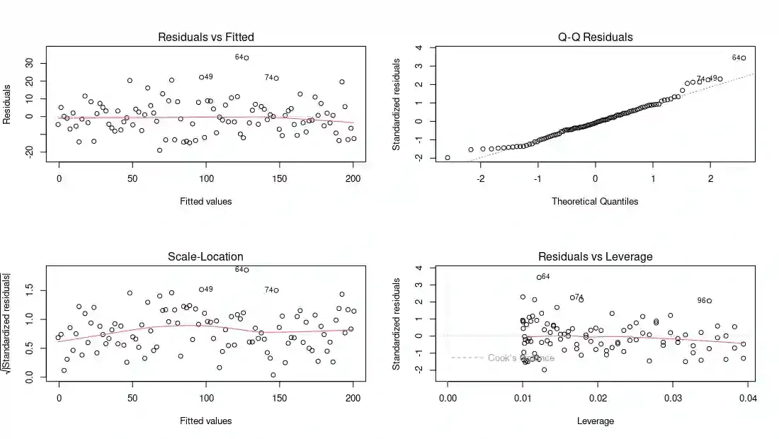
Let's analyze these plots one by one, looking for tell-tale signs of manipulation:
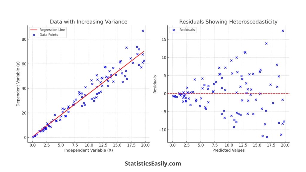
- Residuals vs. Fitted (Top-Left): This plot scatters the residuals against the model's predicted satisfaction scores. We are looking for the absence of any pattern. The red line is a smooth curve through the points; ideally, it should be perfectly flat and near zero. Here, the line is quite flat, and the points are scattered without any obvious shape. This indicates that the linearity assumption holds. However, notice the near-uniform spread of the points. There's no "fanning out" or "funnel" shape, which would indicate non-constant variance (heteroscedasticity). While good, it might almost be too good, like a forger trying too hard to make the errors look random.
-
Normal Q-Q (Top-Right): This plot checks if the residuals follow a normal (Gaussian) distribution. If they do, the points should fall perfectly along the dotted straight line. In our case, the points stick to the line with remarkable precision, especially in the tails. Real-world data rarely exhibits such perfect normality. This is another sign of artificiality; it's as if the "noise" was generated directly from a perfect normal distribution function in a computer program.
-
Scale-Location (Bottom-Left): This is another check for constant variance (homoscedasticity). It plots the square root of the standardized residuals against the fitted values. Again, we are looking for a flat red line, which we see here. The lack of any discernible pattern reinforces the conclusion from the "Residuals vs. Fitted" plot. The variance appears unnervingly constant.
-
Residuals vs. Leverage (Bottom-Right): This plot helps us identify influential data points—cases that have an unusually large impact on the regression coefficients. Points with high leverage (far to the right) and large residuals (far from zero) are potential problems. The dotted red lines show "Cook's distance," a measure of influence. Any point outside these lines would be considered highly influential. Notice that in our plot, all points are well within the acceptable range. There are no outliers or influential points to speak of. A dataset without a single problematic observation is another curiosity.
Taken together, these diagnostic plots do not show violations. Instead, they show a model that is too perfect. The residuals are perfectly normal, their variance is perfectly constant, and there are no influential outliers. This is the statistical equivalent of a crime scene with no dust, no stray hairs, and no fingerprints—a clear sign that it has been cleaned.
The Mind of a Forger
To solidify our case, we must understand the methods and tells of a data forger. What happens to statistical models when data is falsified?
This comprehensive report from the American Association for Public Opinion Research delves into data falsification, including its impact on statistical analyses. It's a field manual for our investigation.
First, read the section on the "Impact on EDA". This will show how falsification can create misleading patterns or, as in our case, potentially mask them. Then, carefully study the section on the "Impact on the Regression Slope". The key takeaway here is the concept of attenuation: when an independent variable is falsified by adding random noise, the estimated regression coefficient is biased towards zero.
The report's finding on attenuation is a crucial piece of the puzzle. It states that falsifying a predictor tends to weaken its observed relationship with the outcome. This means falsification generally leads to lower R-squared values and coefficients that are smaller than the true value.
Our model shows the exact opposite: an incredibly high R-squared. This suggests we are not dealing with a simple case of an interviewer adding random noise to a few survey answers. Instead, it points to a more sophisticated deception: the data was likely generated from a formula. Someone at Elysian Partners decided on a "true" model (e.g., Satisfaction = 5 + 3.5 * Communication + 3 * Activities + error), generated data based on that formula, and then created the Key_Factor_Score as a correlated decoy. This explains both the implausibly high R-squared and the "perfect" residuals.
This practice of manipulating data or analysis to achieve a desired result is a form of scientific misconduct. A fun, quick overview of a related concept, "p-hacking," can help frame this mindset.
The method that can "prove" almost anything - James A. Smith
This TED-Ed video, "The method that can 'prove' almost anything," gives a brilliant and accessible explanation of "p-hacking," where researchers manipulate their analysis to get a statistically significant p-value.
Watch the section that defines p-hacking and its pitfalls. Then, see the concrete example of how researchers used these questionable methods to "prove" that listening to a certain song could make people younger. This illustrates the deceptive mindset we are up against.
The Final Verdict
Our investigation into the fixed survey is now complete. In our previous session, we built a multiple regression model that correctly identified Communication_Frequency and Shared_Activities as the primary drivers of client satisfaction.
Today, we subjected that model to a rigorous forensic analysis. The verdict is clear:
- Extreme Effect Size: The model's R-squared of 0.921 is implausibly high for this type of research, suggesting the data is artificial.
- Sterilized Residuals: The diagnostic plots show residuals that are perfectly normal, perfectly homoscedastic, and free of any outliers. This perfection is a strong indicator of computer-generated data, not real-world observation.
- Contradiction of Attenuation: The typical effect of data falsification is to weaken relationships (attenuation). Our model's extreme strength suggests the opposite: data was likely constructed to fit a clean, theoretical model.
Conclusion: The deception at Elysian Partners runs deeper than we initially thought. They didn't just market a bogus "Key Factor"; they appear to have fabricated their entire dataset to support a narrative of their choosing. They built a house of cards, and our analysis has exposed its foundations as pure fiction.
Preview of the Next Case
With the "Fixed Survey" case closed, a new file lands on your desk. The case comes from a high-end boudoir photography studio that has a major problem: clients are disappearing. After their first session, a significant number of them never book a follow-up or purchase additional products. The studio owner is baffled and needs us to figure out why.
This new mystery requires a different tool from our kit. We are no longer predicting a continuous satisfaction score. Instead, we are predicting a binary outcome: does a client return (Yes/No)? This will lead us into the world of logistic regression, where we will model the probability of an event occurring and identify the key factors that drive a client to disappear.