Visualizing Suspicious Activity with PCA

Greetings, Detective.

In our last session, we took a crucial step in our investigation of the "Anonymous Saboteur." We distilled the tangled web of reviewer data into a handful of potent, underlying patterns—our principal components. We now have a set of "master clues," each one representing a core dimension of reviewer behavior. These components, however, are just abstract directions. To be useful, we must see where they lead us.

Today, we bring our investigation into the visual realm. Our objective is to project the reviewer data onto the principal components and create visualizations to identify clusters of suspicious activity. We will transform our complex dataset into a simple visual "suspect board." By plotting each reviewer in this new space, we will finally be able to see who fits the pattern of normal behavior and, more importantly, who stands out. The saboteur, or saboteurs, may be hiding in plain sight.

The Projection: Placing Reviewers on the Map

The first step is to calculate where each reviewer lands in our new, simplified coordinate system defined by the principal components. This process is called projection. In the last lesson, we identified the eigenvectors of the covariance matrix, which define the directions of our principal components. Now, we will use them to transform our original standardized data.

Mathematically, this is a linear transformation. We take our original standardized data matrix, where each row is a reviewer and each column is a standardized rating attribute, and multiply it by the matrix of our chosen eigenvectors (our principal components).

Let $X_{std}$ be our standardized data and $W$ be the matrix whose columns are the top k eigenvectors we decided to keep. The new, projected data $X_{PCA}$ is calculated as:

X_{PCA} = X_{std} W

The resulting matrix $X_{PCA}$ has the same number of rows (reviewers) but only k columns. Each value in this new matrix is a "score" telling us how much a specific reviewer aligns with a specific principal component.

The following resource provides a clear walkthrough of this entire process, including the final transformation step and its visualization.

Principal Component Analysis (PCA) Made Easy

This guide from Medium provides a complete, hands-on view of the PCA workflow, from the math to the final plots.

First, briefly review the mathematical steps, paying close attention to Step 5, which describes the transformation we're performing. Then, study the geometric interpretation to build your intuition for how this projection works visually. Finally, look at the code examples for both the manual implementation and the scikit-learn implementation. Notice how both end with a scatter plot of the transformed data—this is precisely our goal.

Visualizing the Suspects: The Hunt Begins

With our data projected onto the first two or three principal components, we can now create 2D or 3D scatter plots. Each point on the plot represents a single reviewer, and its position is determined by its scores on the principal components. This visualization is our "suspect board."

By plotting the data this way, we hope to see structures emerge that were invisible in the high-dimensional chaos of the original data. The video below provides an excellent demonstration of how PCA can reveal hidden clusters.

Principal Component Analysis (PCA) Explained Simply

This video from numiqo provides fantastic interactive visualizations of PCA in action.

Focus on the 3D examples. Watch the segment starting around the 3D case, which shows how a messy cloud of points can be simplified. Pay special attention to the example that begins at the next data set, where PCA finds the perfect viewing angle to reveal three distinct clusters. Finally, observe how a real-world dataset is visualized after PCA in the segment from the fun part, where wines are plotted and colored by class, revealing clear groupings.

As the video illustrates, our goal is to find visual patterns. We are looking for two main types of evidence:

Outliers: These are points that lie far away from the main cloud of data. An outlier represents a reviewer whose behavior is highly unusual and not well-described by the dominant patterns. A single, dramatic outlier could be our lone saboteur.
Clusters: These are distinct groups of points that are close to each other but separated from other groups. A tight, isolated cluster of points might represent a coordinated group of saboteurs, like a bot farm, all exhibiting the same fraudulent behavior.

This is the power of projection. As another excellent video explains, projecting onto the principal components is often far superior to projecting onto the original axes for preserving the separability of groups.

Latent Space Visualisation: PCA, t-SNE, UMAP | Deep Learning Animated

This video from Deepia clearly illustrates why the PCA projection is so effective.

Watch the first section of the video, from the beginning until the end of the example. Notice how projecting the data onto the principal component successfully preserves the three-cluster structure, whereas projecting onto the original x-axis merges two of the clusters, destroying critical information.

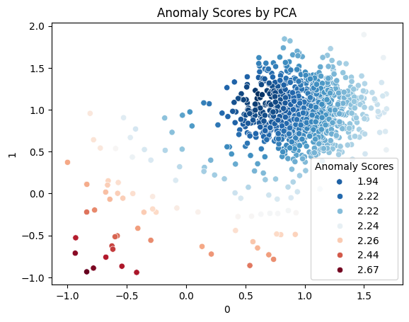
The image below shows exactly what we're hoping to find: a visualization of our reviewers where the patterns are clear.

This 3D scatter plot shows data projected onto three principal components. Notice how two distinct clusters of "normal" behavior are revealed, along with a single, highly suspicious anomaly point that stands apart from everyone else. This is a primary suspect.

Quantifying Suspicion: The Residual Score

Visual inspection is a powerful tool, but we can support our detective work with a more quantitative measure of suspiciousness. Recall from our last lesson that PCA separates our data's variance into a few important components and many unimportant ones. The space spanned by the top components (e.g., PC1, PC2) is called the normal subspace, as it describes typical behavior. The space spanned by the remaining, discarded components is the residual subspace.

The core idea is this: a normal reviewer's behavior should be well-explained by the principal components. A saboteur's behavior, however, might deviate in ways that are not captured by these main patterns. Their behavior will have a large "residual" component that lies outside the normal subspace.

We can calculate an anomaly score (often called the Squared Prediction Error or SPE) for each reviewer. This score is the squared magnitude of the part of their data that lies in the residual subspace. A high anomaly score means the reviewer's behavior is not well-represented by the common patterns in the data, making them highly suspicious.

The following academic paper, which uses PCA to detect fake users in social networks, formalizes this exact technique.

[PDF] Towards Detecting Anomalous User Behavior in Online Social ...

This research paper provides a rigorous foundation for using PCA as an anomaly detection tool, a perfect fit for our investigation.

Read the section titled Detecting Anomalous User Behavior. You'll recognize the projection formula. The key insight is the separation of a user's behavior vector x into a normal portion x_n and a residual portion x_r. The logic that "if ||x_r||^2_2 is unusually large... then x is likely anomalous" is the quantitative backbone of our search for the saboteur.

By calculating this score for every reviewer, we can create a plot where points are colored by their anomaly score, immediately drawing our eye to the most suspicious individuals.

A 2D PCA plot where each point represents a user. The color indicates the user's anomaly score, with darker, redder points being more anomalous. This visualization allows a detective to immediately focus on the most suspicious individuals, like those in the bottom left corner.

Conclusion

Today, we have turned our abstract statistical components into a concrete investigative tool. We've learned how to project our high-dimensional data into a low-dimensional space and create visualizations that act as a "suspect board." By looking for outliers and distinct clusters, we can now visually identify individuals whose behavior deviates from the norm.

Key Takeaways:

Projection is the process of transforming the original data into the new coordinate system defined by the principal components, giving each data point a "score" on each component.
Visualizing the projected data in 2D or 3D scatter plots can reveal hidden structures, such as clusters of similar reviewers and anomalous outliers.
Outliers (points far from the main data cloud) and isolated clusters are primary targets in our search for the saboteur.
We can quantify suspicion by calculating an anomaly score based on the data's projection onto the residual subspace. A high score indicates behavior that is not well-explained by normal patterns.

Preview of the Next Lesson

Our visual analysis has been incredibly fruitful. We have a list of individual outliers and, potentially, one or more suspicious clusters of reviewers. These clusters are our strongest lead yet, suggesting a coordinated effort. However, simply eyeballing them on a plot isn't enough. We need to formally identify who belongs to which group.

In our next session, we will move from visual inspection to algorithmic grouping. We will learn how to apply hierarchical clustering methods to our reduced dataset. This will allow us to systematically group the suspects and understand the structure of their conspiracy, bringing us one step closer to unmasking the anonymous saboteur.

Recommended resources