Greetings, Detective.
In our last briefing, we successfully projected our high-dimensional reviewer data onto a "suspect board," revealing the hidden patterns of behavior through Principal Component Analysis. The resulting scatter plots were illuminating, showing us not just lone-wolf outliers but also distinct clusters of reviewers acting in concert. This visual evidence strongly suggests a coordinated effort, a conspiracy.
However, simply circling groups on a chart is not enough to build a case. We need a formal, systematic method to define the structure of this conspiracy. Today, our objective is to group the suspects by applying and comparing both single-linkage and complete-linkage hierarchical clustering methods to the reduced data. We will move from visual intuition to algorithmic precision, constructing a detailed "family tree" of our saboteurs. By comparing two different methods for building this tree, we can see the conspiracy from different angles and better understand its internal structure.
From Individuals to Syndicates: Hierarchical Clustering
The core idea we'll use is agglomerative hierarchical clustering. Think of it as building a case from the ground up. We start by treating each of our suspects as an individual "cluster" of one. Then, we follow a simple, iterative process:
- Find the two closest clusters (individuals or groups).
- Merge them into a single, new cluster.
- Repeat until all suspects are grouped into one large syndicate.
This entire process of mergers is visualized in a tree-like structure called a dendrogram, which serves as our definitive organizational chart of the saboteur network. The following video provides a superb, intuitive introduction to this concept.
StatQuest: Hierarchical Clustering
This StatQuest video with Josh Starmer is excellent for building a conceptual foundation for what we're about to do.
Watch the first two parts of the video. The first part, up to the start of the example, introduces the idea of clustering, dendrograms, and how they bring order to data. Then, watch the main procedural explanation from the step-by-step example, which walks through the iterative merging process and shows how the dendrogram is built.
As the video explains, the key steps involve measuring similarity (or distance), merging the most similar items, and repeating the process. But this raises a crucial question: how do we measure the distance between two clusters of suspects, especially when they contain multiple individuals? The answer lies in the linkage method.
Interrogation Tactics: Single vs. Complete Linkage
The linkage method is the rule that defines the distance between two clusters. Today, we'll investigate two fundamental "interrogation tactics" to uncover the structure of our suspect groups.
1. Single Linkage: The Nearest Neighbor Approach
This method defines the distance between two clusters as the distance between the closest pair of individuals, with one from each cluster. It's an optimistic method, looking for any link, no matter how tenuous, to connect two groups.
- Formula:
- Effect: This tends to produce long, "stringy" clusters. It can chain together distant groups if there's a path of intermediate individuals connecting them. In our case, this could reveal a sprawling, loosely-affiliated network with many degrees of separation.
2. Complete Linkage: The Farthest Neighbor Approach
This method takes the opposite approach. It defines the distance between two clusters as the distance between the farthest pair of individuals. It's a conservative method, ensuring that all members of a potential new cluster are relatively close to one another before merging.
- Formula:
- Effect: This tends to produce tight, compact, roughly spherical clusters. It's excellent for identifying core, close-knit cells within the conspiracy where all members are highly similar to each other.
The video below explains these two contrasting approaches with clear examples.
IAML19.5 Single-link, complete-link, Ward's method
This lecture excerpt from Victor Lavrenko provides a concise mathematical and visual explanation of single and complete linkage.
First, watch the explanation of single linkage, paying attention to how the minimum distance is used to decide which clusters to merge. Then, watch the section on complete linkage, which contrasts this by using the maximum distance and explains its effect on creating more "spherical" clusters.
The Case File: A Step-by-Step Reconstruction
To truly understand how these methods work, let's walk through the process by hand. Your background in operations research and algorithms will make this step-by-step procedure very familiar. We will use a small dataset of 5 "suspects" with their positions in our 2D PCA space.
The following guide provides a perfect, detailed walkthrough. We'll follow its steps to build the dendrograms for both single and complete linkage.
The complete guide to clustering analysis: k-means and hierarchical ...
This guide from statsandr.com provides an excellent manual calculation for hierarchical clustering. We'll use it to work through the mechanics.
Begin at the section "Application 3: hierarchical clustering". First, read the subsections Data and Solution by hand to understand the initial setup and the calculation of the starting distance matrix. This matrix is our primary piece of evidence. Next, carefully follow the entire Single linkage section. Note how at each step, the algorithm finds the smallest distance in the current matrix to decide the merge, and then uses the minimum rule to update the distances for the newly formed cluster. Finally, read the Complete linkage section. Pay close attention to how the procedure is identical except for the rule used to update the distance matrix after a merge—here, it uses the maximum distance between the original points.
By working through this example, you've seen firsthand how the choice of linkage criterion directly impacts the structure of the resulting hierarchy and the merge heights on the dendrogram.
Comparing the Evidence
Now that we understand the mechanics, let's look at the results. Different linkage methods can lead to very different conclusions about how our suspects are organized.
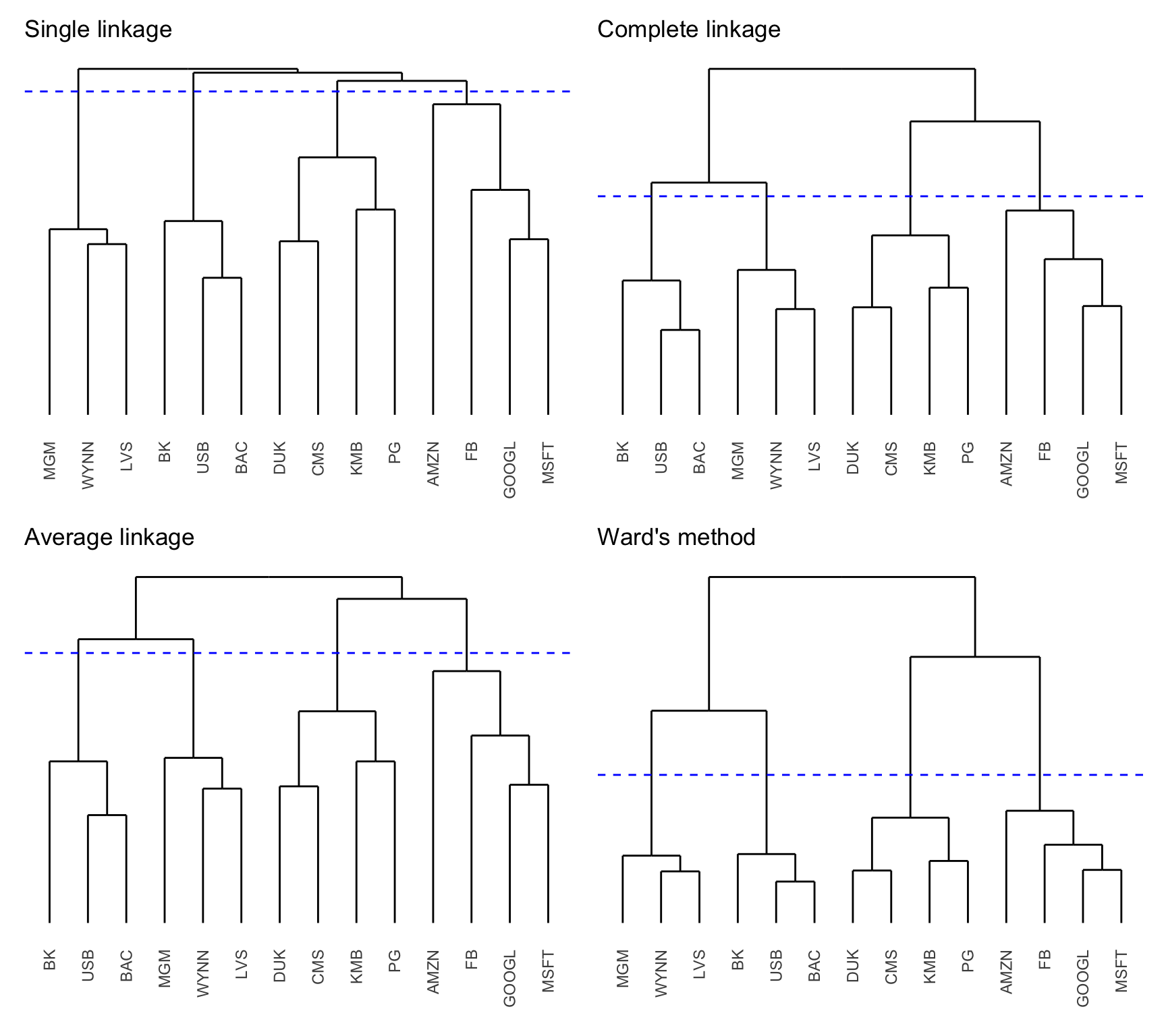
The image above shows how four different methods, including single and complete linkage, group a set of stocks. With single linkage, items are added one-by-one, creating a chain. With complete linkage, more balanced, distinct groups are formed. In our investigation, single linkage might connect a central "mastermind" to their operatives through a series of intermediaries, while complete linkage would be better at identifying distinct, self-contained cells of saboteurs.
The choice of method depends on the underlying structure of the data you expect to find.
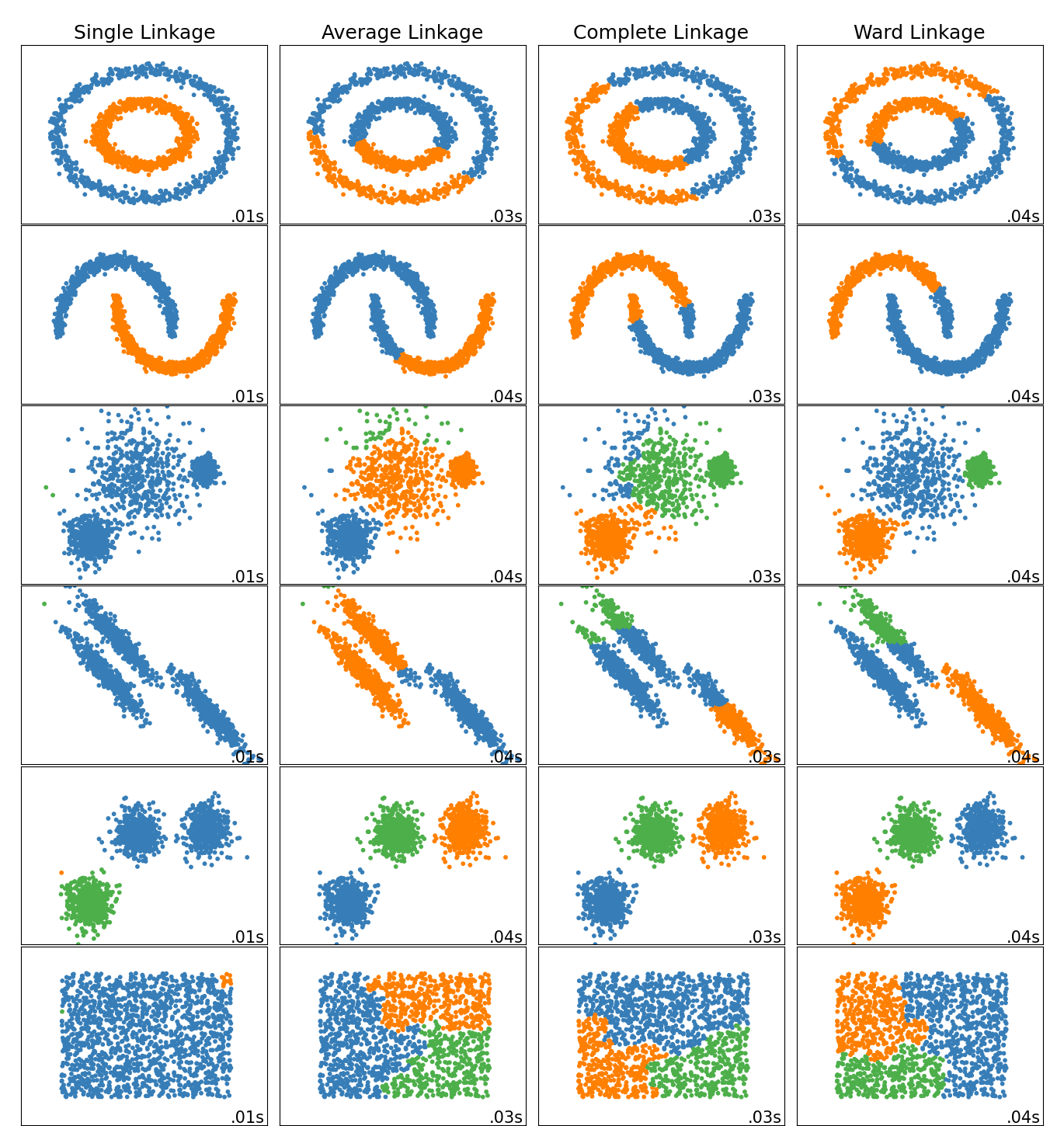
This image is particularly insightful.
- Row 1 (Nested Circles): Notice how only Average and Ward linkage perform reasonably well. Single linkage connects the two rings, and complete linkage splits them incorrectly.
- Row 2 (Moons): Single linkage is the clear winner here, as its ability to follow the "chain" of points allows it to correctly separate the two crescent shapes.
- Row 3 & 4 (Blobs with Noise/Variance): Complete and Ward's methods excel at carving out clean, compact clusters, whereas single linkage is easily fooled by the "bridge" of noise between the groups.
This tells us that there is no single "best" method. A smart detective applies multiple methods to see which story best fits the evidence. For our saboteur case, running both single and complete linkage will help us see if we're dealing with a single, sprawling network (which single linkage would reveal) or multiple, tight-knit cells (which complete linkage would identify).
Conclusion
We have now added a powerful set of algorithmic tools to our investigative arsenal. Instead of just visually inspecting our PCA plots, we can now formally and systematically group our suspects. This process not only identifies the members of each conspiratorial cell but also reveals the hierarchical structure that binds them together.
Key Takeaways:
- Hierarchical Clustering is an agglomerative method that builds a tree of clusters (a dendrogram) from the bottom up, starting with individual data points.
- Linkage Methods define how the distance between clusters is measured.
- Single Linkage uses the minimum distance between points in two clusters. It is effective for discovering non-globular, chain-like structures but can be sensitive to noise.
- Complete Linkage uses the maximum distance between points. It tends to find compact, spherical clusters and is less sensitive to noise but may fail to identify more complex shapes.
- Comparing the results of different linkage methods provides a more robust understanding of the underlying patterns in the data.
Preview of the Next Lesson
This lesson marks the conclusion of our investigation into "The Anonymous Saboteur." We have successfully used dimensionality reduction and clustering to move from a chaotic dataset to a clear picture of the individuals and groups responsible for the sabotage.
In our next case, "The Mystery Client," we face a new challenge. We will be given the profile of a single, unknown individual and tasked with predicting their behavior. This will require us to shift gears from unsupervised learning (finding patterns in data) to supervised learning (making predictions based on labeled examples). Our first task will be to classify this mystery client using their nearest neighbors, employing a technique you may already know: the K-Nearest Neighbors algorithm.