Dimensionality Reduction with PCA

The Art of Synthesizing Clues

At its heart, Principal Component Analysis is a method for synthesizing information. Imagine our reviewer data as a cloud of points in a high-dimensional space, where each dimension is a review attribute like 'fit', 'fabric', 'style', etc. PCA finds a new set of coordinate axes to describe this cloud.

The key is that these new axes, called principal components (PCs), are chosen very strategically:

1. The first principal component (PC1) is oriented in the direction of the greatest variance in the data. It's the single line that best captures the spread of all the points.
2. The second principal component (PC2) is oriented to capture the most of the remaining variance, with the crucial constraint that it must be orthogonal (perpendicular) to PC1.
3. This process continues for each subsequent component, each one capturing the maximum remaining variance while being orthogonal to all the ones before it.

This process is like rotating our perspective on the data cloud until we find the most informative view.

By doing this, we create new, "synthetic" variables that are uncorrelated linear combinations of the original ones. Often, the first few principal components capture the vast majority of the information (variance) in the original dataset. This is the essence of dimensionality reduction: we can describe our data with fewer, more meaningful variables without significant loss of information.

The video below offers an excellent, practical explanation of this concept.

The Engine Room: Eigenvalues and Eigenvectors

So, how does PCA find these magical new axes? The answer lies in the eigen-decomposition of the covariance matrix we calculated in our last session. Given your background in statistics, you'll recognize this as a cornerstone of multivariate analysis.

For our covariance matrix, let's call it $\mathbf{C}$, the eigen-decomposition finds sets of eigenvalues ($\lambda$) and eigenvectors ($\mathbf{v}$) that satisfy the equation:

In the context of PCA, these have very specific and powerful interpretations:

• Eigenvectors ($\mathbf{v}$): Each eigenvector defines the direction of a principal component. It's a vector of weights, called loadings, where each weight corresponds to an original variable. These loadings tell us how the original variables are combined to form that principal component. The eigenvector corresponding to the largest eigenvalue defines PC1, the second largest defines PC2, and so on.
• Eigenvalues ($\lambda$): Each eigenvalue represents the amount of variance captured by its corresponding eigenvector (principal component). A large eigenvalue means its component accounts for a significant portion of the information in the data.

Therefore, by finding the eigenvalues and eigenvectors of our covariance matrix, we are simultaneously finding the importance ($\lambda$) and direction ($\mathbf{v}$) of our new, optimal axes.

The following guide walks through the entire PCA process, connecting all the steps we've discussed.

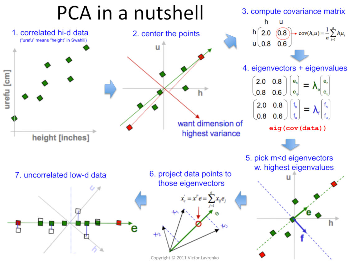
A Step-by-Step Investigation

Let's formalize the procedure. The resource below provides a detailed breakdown of the steps, which we'll follow in our investigation.

As you've just read, the process can be summarized as follows:

1. Standardize the Data: We've already done this. Our data has a mean of 0 and a standard deviation of 1 for all attributes.
2. Calculate the Covariance Matrix: We've also done this. This matrix, $\mathbf{C}$, is the input for the next, crucial step.
3. Perform Eigen-decomposition on $\mathbf{C}$: We calculate the eigenvalues and eigenvectors.
4. Sort and Select Components: We sort the eigenvalues in descending order. This automatically ranks our principal components from most to least important.
5. Project the Data: We use the selected eigenvectors to transform our original standardized data into the new principal component space.

The following resource provides a numerical example of steps 3-5.

How Many Components Are Enough?

A key decision in our investigation is choosing how many principal components to retain. If we keep all of them, we've simply rotated the data without reducing its dimensionality. If we keep too few, we risk throwing away valuable information. There are two common methods for making this decision:

1. The Scree Plot: This is a bar chart of the eigenvalues (or the proportion of variance they explain) in descending order. We typically look for an "elbow" in the plot—the point where the variance explained by subsequent components drops off sharply. Components before the elbow are generally retained.

2. Cumulative Variance Explained: We calculate the cumulative proportion of variance explained by the components. A common heuristic is to keep enough components to explain a high percentage of the total variance, such as 80% or 90%.

The video below excellently demonstrates both the scree plot and the concept of loadings, which are essential for interpreting our results.

By applying these methods, we can confidently reduce our dozens of review attributes to perhaps 2, 3, or 4 principal components, creating a manageable yet powerful dataset that captures the essence of reviewer behavior. These components—like "General Quality Score," "Aesthetic vs. Practical," or "Price Sensitivity"—will be the new axes for our investigation.

Conclusion

Today, we've moved from a complex map of correlations to a streamlined set of investigative leads. We've uncovered the theoretical underpinnings of Principal Component Analysis, understanding it as a process of rotating our data to find the directions of maximum information. By performing an eigen-decomposition of the covariance matrix, we have extracted these principal components.

Key Takeaways:

• PCA reduces dimensionality by creating new, uncorrelated variables called principal components that are linear combinations of the original variables.
• The directions of the principal components are given by the eigenvectors of the covariance matrix.
• The amount of variance explained by each component is given by its corresponding eigenvalue.
• The first principal component (PC1) captures the most variance, PC2 captures the most remaining variance (and is orthogonal to PC1), and so on.
• We can decide how many components to keep by using a scree plot or by setting a threshold for the cumulative variance explained.

Preview of the Next Lesson

We have successfully distilled the sprawling reviewer data into a few potent "super-variables." We now have a low-dimensional representation that we believe captures the most important patterns of behavior. But the saboteur is still hiding.

In our next session, we will take our newly transformed data and bring it to life. We will project the reviewer data onto the principal components and create visualizations. By plotting the reviewers in this new, simplified space, we will hunt for outliers and suspicious clusters. This visual analysis will be our next major step in tracking down the anonymous saboteur.