Simplifying Complexity: PCA for Behavioral Data

The Problem of Too Much Information: The Curse of Dimensionality

In our line of work, you'd think more information is always better. However, when building a profile or a predictive model, adding more and more features (or "dimensions") can paradoxically make things worse. Past a certain point, new features add more noise than signal, confusing our analysis and hiding the very patterns we seek. This phenomenon is known as the curse of dimensionality.

Imagine trying to profile a suspect. You start with key variables: age, location, income. Your profile is clear. Then you add shoe size, favorite color, preferred coffee shop, number of social media posts per day, average review length... soon you have hundreds of variables. Instead of a sharp profile, you have a blurry mess. Your model, or your own expert judgment, gets bogged down in irrelevant details.

To get a more formal intuition for this, we'll turn to a short video explanation.

As the video explains, we have two main ways to combat this:

1. Feature Selection: We could try to pick the "most important" variables and discard the rest. This is risky, as we might throw away features that seem unimportant alone but are crucial in combination.
2. Feature Extraction: We can create a smaller set of new, synthetic features from the old ones, with the goal of retaining as much of the original information as possible.

It is this second approach, feature extraction, that we will employ today. We don't want to throw away data; we want to transform it into a more manageable and insightful form.

A New Perspective: Principal Component Analysis (PCA)

The tool for this job is Principal Component Analysis (PCA). PCA is not a data reduction technique in itself, but a data transformation technique. It doesn't discard variables; it reframes the entire dataset, creating a new coordinate system based on the patterns within the data itself.

PCA constructs new variables, called principal components (PCs), which are weighted sums of the original variables. The magic of PCA is how it constructs them:

• The first principal component (PC1) is oriented in the direction of the largest possible variance in the data. It is the single most informative summary of the data.
• The second principal component (PC2) is orthogonal (at a right angle) to the first and captures the next largest amount of variance.
• This continues for as many dimensions as you started with, with each successive component capturing less and less of the remaining variance.

By transforming our data onto these new axes, we concentrate the most important information into the first few components, allowing us to see the primary patterns of activity.

The Geometry of Insight

Let's visualize this. Imagine our behavioral data has only two features, say review_frequency (X-axis) and purchase_frequency (Y-axis). The data points might form an elongated cloud. Neither axis alone tells the full story.

PCA finds the line that passes through the center of this cloud and best captures its spread. This line is our first principal component (PC1). The line perpendicular to it is the second (PC2).

By rotating our view to align with these new axes, the underlying structure of the data becomes clear.

The Engine Room: Eigen-decomposition of the Covariance Matrix

Given your background in statistics, we can look under the hood at the mechanism that finds these principal components. The process relies on concepts you're familiar with: standardization, covariance matrices, and eigen-decomposition.

1. Standardize the Data: Before PCA, we must standardize each variable to have a mean of 0 and a standard deviation of 1. This is crucial because PCA is sensitive to the scales of the original variables. A variable with a large range (e.g., time_spent_on_forums in seconds) would dominate the analysis over a variable with a small range (e.g., average_review_score from 1-5), regardless of its actual importance. Standardization puts all variables on equal footing.

2. Compute the Covariance Matrix: Next, we compute the covariance matrix for our standardized data. This $p\times p$ matrix (where $p$ is the number of features) summarizes the variance of each feature and the covariance between each pair of features.

3. Calculate Eigenvectors and Eigenvalues: Here is the core of PCA. The principal components are the eigenvectors of the covariance matrix, and the variance explained by each principal component is its corresponding eigenvalue.

   • The eigenvector with the largest eigenvalue is the first principal component (PC1). It points in the direction of maximum variance.
   • The eigenvector with the second-largest eigenvalue is the second principal component (PC2), and so on.

This mathematical property is what allows PCA to systematically find the new axes that capture the most information.

A scientific paper on applying PCA to robotic assessment data provides a concise summary of the standard procedure, confirming these steps.

Interpreting the Clues: Explained Variance and Loadings

After running PCA, we are left with a new set of principal components. To use them in our investigation, we need to interpret two key outputs.

1. Explained Variance and the Scree Plot

The eigenvalue of each PC, when divided by the sum of all eigenvalues, gives us the proportion of variance explained by that component. We can plot these values in a scree plot, which helps us decide how many components are needed to capture most of the information in the data. A common practice is to keep enough components to explain 90%, 95%, or even 99% of the total variance.

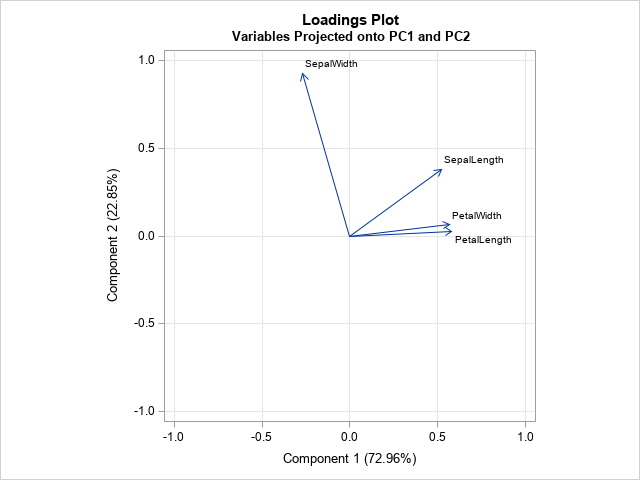
2. Component Loadings

To understand what each principal component represents, we examine its loadings. The loadings are the correlation coefficients between the original variables and the principal component. A variable with a high loading (close to +1 or -1) on a PC contributes strongly to it. By looking at which variables load highly onto a component, we can assign it a meaningful, interpretable label. This is how we isolate the significant patterns of activity.

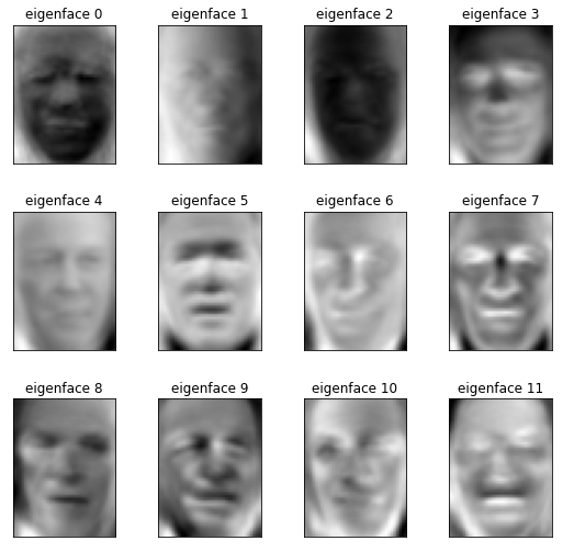
A classic, striking example of PCA's power is its application to image analysis, resulting in "eigenfaces".

Back to the Case

Now, let's apply this to our mastermind investigation. We have dozens of behavioral variables. After running PCA, we might find that the first three components explain 90% of the variance. We can then focus our analysis on just these three components.

By examining the loadings, we could find:

• PC1 (The "Agitator"): High positive loadings for forum_post_frequency, negative_review_count, and high negative loading for average_purchase_value.
• PC2 (The "Influencer"): High positive loadings for social_media_follower_count, loyalty_program_points, and boutique_visit_frequency.
• PC3 (The "Shadow Broker"): High positive loadings for use_of_anonymizing_proxies, transaction_amount_variability, and high negative loading for account_age.

Instead of juggling 30+ variables, we now have three intuitive behavioral archetypes. We can score each of our suspects on these three components and plot them in this new 3D space. The mastermind will no longer be lost in the noise; their unique behavioral signature will stand out.

Conclusion

You've now been equipped with a powerful technique for navigating high-dimensional data. PCA allows us to cut through overwhelming complexity and find the underlying structure. By transforming our data into a new space defined by principal components, we can reduce dimensionality while preserving the crucial information carried in the variance. Interpreting the explained variance tells us how much information each component holds, while the loadings tell us what that information is.

Key Takeaways:

• High-dimensional data can suffer from the curse of dimensionality, where excess features obscure patterns and degrade model performance.
• Principal Component Analysis (PCA) is a feature extraction technique that transforms data onto a new coordinate system of principal components.
• Each successive PC captures the maximum possible remaining variance and is orthogonal to the previous ones.
• The process involves standardizing data, computing the covariance matrix, and finding its eigenvectors (the PCs) and eigenvalues (the variance explained).
• We use a scree plot of explained variance to decide how many components to retain for our analysis.
• We interpret the meaning of each PC by examining the loadings, which are the correlations between the original variables and the new component.

Preview of the Next Lesson

We have successfully transformed our noisy, complex behavioral data into a simplified, interpretable map defined by a few key patterns of activity. Our suspects are no longer just rows in a sprawling spreadsheet; they are points in a new "behavioral space". In our next session, we will use this map to hunt for our mastermind. We will apply clustering algorithms to this reduced data to segment our suspects into distinct groups, allowing us to isolate the most suspicious cluster and narrow our search.