Greetings, Detective.
Our investigation into the "Midnight Seraph" inventory has borne fruit. By establishing the correct reorder point, we uncovered our first concrete piece of evidence: three sets of lingerie vanished from a single order cycle, not sold, simply gone. This is more than a clerical error; it's a footprint. But a single footprint doesn't tell us the size of the beast. Was this a one-time slip-up or part of a larger, systematic heist? Our adversary is clearly clever enough to manipulate the inventory system, but how deep does the deception go?
In our previous sessions, we established the financial blueprint for a perfectly run operation: an Economic Order Quantity (EOQ) of 60 units should result in a minimum annual inventory cost of $3,000, based on the official annual demand of 1,200 units. Today, we will weaponize this blueprint. We will explore how sensitive this optimal cost is to the very data we've been given. What if the demand figures themselves are a lie? By systematically testing different "what-if" scenarios, we can reveal the true scale of the manipulation and translate the boutique owner's vague feelings of financial strain into a quantifiable estimate of the damage.
The "What-If" Machine: Sensitivity Analysis
In operations research, we don't just find an answer; we test its resilience. This is the purpose of sensitivity analysis. It's a formal way of asking "what if our assumptions are wrong?" By changing the input parameters of a model—like demand, ordering cost, or holding cost—we can observe the effect on the optimal solution and the total cost.
This is an invaluable tool for a detective. It allows us to model different criminal hypotheses and see which one best fits the evidence on the ground. A short paper, "Sensitivity analysis applied to a collaborative inventory model," provides a concise definition.
[PDF] Sensitivity analysis applied to a collaborative inventory model
This paper introduces the concept of sensitivity analysis in the context of inventory management. It will help formalize our investigative approach.
Read the section on "Literature review," focusing on the definition of sensitivity analysis and its purpose. Also, note the example by Basri, who uses it to explain various scenarios—exactly what we are about to do.
The core of our analysis rests on the two foundational formulas for the EOQ model:
Total Annual Cost (TC):
Economic Order Quantity (EOQ or Q*):
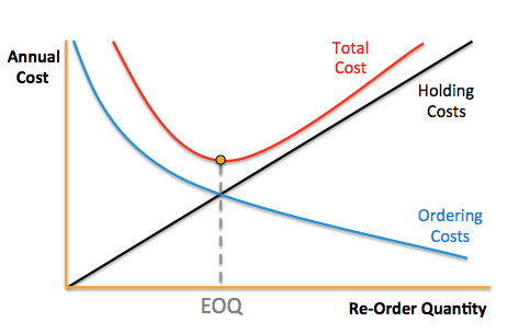
As you can see, both the total cost and the optimal order quantity are functions of annual demand (D), ordering cost (S), and holding cost (H). Our intelligence has established S = $75 per order and H = $50 per unit per year. The only variable in question is D, the annual demand. The graph below illustrates the balance we're investigating.
A brief video will quickly demonstrate qualitatively how changes in these parameters affect the EOQ.
This clip from a lecture by POM ETH Zurich provides a succinct visual and verbal explanation of the EOQ formula's sensitivity.
Watch the segment from the discussion of external factors. Pay close attention to the final point: what happens when demand drops? This is the lever we will be pulling in our own analysis.
Modeling the Crime: Two Scenarios
The discrepancy we found could be the result of two primary methods of manipulation. Let's model them both.
Scenario A: Under-Reported Demand (Cash Skimming)
In this scenario, the thief is a trusted employee who handles sales. They sell a "Midnight Seraph" set, pocket the cash, and simply delete the transaction from the sales records.
- Effect: The true demand (actual number of units leaving the store) is higher than the reported demand in the accounting system.
- Symptom: The boutique owner feels a constant financial squeeze. Costs seem higher than they should be, and cash flow is tight, even though the books look balanced.
Let's quantify this. The boutique operates based on the reported demand of D = 1,200 units, so they order the EOQ of Q = 60 units each time. But what if the true demand is, say, 20% higher at D' = 1,440 units?
Because they are satisfying a higher demand (1,440 units) but ordering in suboptimal batches of 60, their actual annual cost will be:
The annual cost has inflated from the expected $3,000 to $3,300. This $300 "cost penalty" is a direct financial symptom of the theft, not including the value of the stolen goods themselves. The boutique is paying more for inventory management because its ordering policy is out of sync with reality.
This next video segment demonstrates exactly this effect: how ordering a quantity different from the true EOQ always results in a higher total cost.
Economic Order Quantity (EOQ) in Inventory Management
This video, "Economic Order Quantity (EOQ) Explained," provides a detailed example of what happens when you are forced to order a quantity that is not the calculated EOQ.
Watch the "curveball" example from the explanation of non-EOQ orders. Notice how the total cost increases when the order quantity deviates from the optimal 300 units. This is precisely what happens in our cash-skimming scenario: the boutique orders 60 units, but the true optimal quantity for the higher demand would be different.
Scenario B: Over-Reported Demand (Direct Theft)
In this scenario, the thief simply steals physical boxes of lingerie. To cover their tracks, they inflate the sales numbers in the system.
- Effect: The reported demand is higher than the true customer demand.
- Symptom: The primary complaint isn't about cost, but about "phantom inventory." The system says there are units on the shelf that aren't physically there, leading to constant, frustrating stock-outs and write-offs during physical counts.
Let's model this. Suppose the true customer demand is D = 1,200, but the thief has inflated the records to show D' = 1,440 units to cover the theft of 240 units over the year. The boutique manager, seeing the inflated demand, calculates a new, "optimal" order quantity:
So, they start ordering in batches of 66. However, their costs are driven by the real customer demand of 1,200 units.
Notice that the total inventory cost is barely above the optimal $3,000. This is because the total cost curve is relatively flat near the minimum. In this scenario, the financial signal is extremely weak. The real evidence is the massive inventory discrepancy: the system thinks 1,440 units were sold, but customers only bought 1,200. The difference—240 units—is the amount stolen.
Quantifying the Scale of the Heist
We can now build a sensitivity table to present to the boutique owner. This allows us to connect a financial symptom (excess cost) to a specific level of theft.
| Scenario A: True Demand vs. Reported Demand (1,200 units) |
| :--- | :---: | :---: | :---: |
| True Annual Demand | 1,200 (Baseline) | 1,320 (+10%) | 1,440 (+20%) |
| Annual Units Sold Off-the-Books | 0 | 120 | 240 |
| Actual Annual Cost (Ordering Q=60) | $3,000 | $3,150 | $3,300 |
| Cost Penalty vs. Baseline | $0 | +$150 | +$300 |
This table is our forensic tool. If the boutique's accountant confirms that annual inventory costs are running approximately $300 higher than projected, we can confidently assert that the problem is likely cash skimming, and the scale is roughly 240 units per year, or about 20% of the legitimate business. The article "A study on inventory management" uses similar tables to show these relationships.
[PDF] A study on inventory management with a reference to EOQ model
This paper provides simple, clear tables demonstrating sensitivity analysis, which serves as a model for our own report.
Look at Table 1 and Table 2. These tables show how the EOQ value changes as demand and costs are altered. Our table does something similar, but focuses on the impact on total cost when the order quantity is fixed at a suboptimal level due to manipulated data.
Conclusion
We have now moved from detecting a crime to quantifying its scale and diagnosing its method. Sensitivity analysis has allowed us to translate abstract financial data into concrete criminal scenarios. We've seen that different methods of theft leave different signatures: cash skimming creates a clear financial trail of increased costs, while direct theft creates an operational trail of phantom inventory.
By asking the right "what-if" questions, we have built a powerful analytical tool. The next step in any investigation is to present the findings. Armed with this analysis, we can explain to the boutique owner not just that they are being robbed, but how, and by how much.
Key Takeaways:
- Sensitivity analysis is a "what-if" technique used to measure how changes in a model's parameters (like demand) affect its outputs (like total cost).
- By modeling different theft scenarios, we can identify their unique financial and operational signatures.
- Cash Skimming (Under-reported Demand): Leads to a noticeable increase in total annual inventory costs because the ordering policy is mismatched with the higher true demand.
- Direct Theft (Over-reported Demand): Leads to a negligible change in inventory costs but creates a large discrepancy between physical and recorded inventory.
- The results of a sensitivity analysis can be presented in a table to clearly link a symptom (e.g., a specific cost increase) to the scale of the problem (e.g., number of units stolen).
Preview of the Next Lesson
We have successfully diagnosed and quantified a localized heist at a single boutique. However, intelligence suggests this may be part of a much larger, more sophisticated operation spanning multiple businesses, orchestrated by a single mastermind. To tackle this, we will need to graduate from analyzing a single product line to sifting through vast, complex behavioral datasets. In our final case, "The Mastermind's Gambit," we will employ advanced techniques like dimensionality reduction and clustering to uncover hidden patterns, identify suspect groups, and ultimately build a profile of the ringleader behind it all.