Welcome back, Detective.
In our last session, we took the chaotic digital footprint of our suspects—a dizzying array of over 30 behavioral variables—and tamed it. Using Principal Component Analysis, we collapsed that high-dimensional mess into a clean, two-dimensional "map". Each suspect is now a single point on this map, their position defined by their scores on our new axes: PC1, the "Agitator" score, and PC2, the "Influencer" score. The noise has been silenced.
But a map is only useful if you know what to look for. Our mastermind isn't acting alone. They have a crew, an inner circle who likely share similar behavioral patterns. On our new map, these individuals should appear grouped together, forming distinct behavioral cells. Today, our mission is to find these groups. We will apply powerful grouping techniques to our reduced data, moving from a scatter of individual points to a clear segmentation of our suspects. By identifying these clusters, we can isolate the most anomalous and coordinated group—the likely hideout of our mastermind.
The Art of Finding Gangs in Data
The task of automatically grouping similar objects is known as clustering. It's a cornerstone of unsupervised learning, meaning we don't tell the algorithm what the groups are ahead of time; we ask it to discover the natural groupings within the data.
In our case, the "objects" are our suspects, and their "features" are their scores on the principal components we derived. We want to partition these suspects so that individuals within the same group are very similar to each other (in terms of their "Agitator" and "Influencer" scores), and very different from individuals in other groups.
Clustering on Principal Component Analysis - Charles Holbert
This blog post by Charles Holbert provides a concise introduction to the idea of combining PCA and clustering, which is precisely our strategy.
Read the short Introduction section. It frames the exact two-step process we are undertaking: first reduce dimensionality with PCA, then perform cluster analysis on the results.
We will explore two primary methods for this task: K-Means Clustering and Hierarchical Clustering.
Method 1: K-Means Clustering - Finding the Centers of Gravity
K-Means is one of the most popular and intuitive clustering algorithms. Imagine our PCA map of suspects. K-Means tries to find a pre-specified number of "cluster centers" (called centroids) and assigns each suspect to the nearest center.
To build your intuition, let's use an analogy.
How to Group an Audience by Personality Traits Using ...
This article from Receptiviti uses a simple, effective analogy to explain K-Means.
Read the section under the heading "K-means Clustering with LEGOs". Think of our suspects as the LEGOs and their behavioral profiles (their PC scores) as the characteristics like color and shape.
The process described in the LEGO analogy is iterative. The algorithm doesn't get it right on the first try. It refines the clusters step-by-step until the groupings are stable.
This video provides an excellent visual demonstration of that iterative process.
Hands On Data Science Project: Understand Customers with KMeans Clustering in Python
In this project-based tutorial, "Hands On Data Science Project: Understand Customers with KMeans Clustering," the channel TrentDoesMath visually walks through the K-Means algorithm.
Watch the segment from the visual explanation of the algorithm. Observe how the centroids (the red 'x's) are initialized randomly and then iteratively move to the center of their assigned data points until they stabilize. This is the core mechanic of K-Means.
The Crucial Question: How Many Clusters?
The "K" in K-Means is the number of clusters we want to find. This is a parameter we must choose. How do we decide how many "crews" our suspects have formed? Two, three, five? Choosing the right K is critical. We use a combination of quantitative metrics and expert judgment.
-
The Elbow Method: We can run the K-Means algorithm for a range of different K values (e.g., from 2 to 10 clusters) and for each run, we measure the inertia. Inertia is the sum of squared distances of samples to their closest cluster center. As K increases, inertia will always decrease. However, we look for an "elbow" in the plot of inertia vs. K—the point where adding another cluster stops providing a significant drop in inertia. This suggests we are hitting a point of diminishing returns.
-
The Silhouette Score: This metric evaluates how well-separated the clusters are. For each data point, it measures how similar it is to its own cluster compared to other clusters. The score ranges from -1 to +1, where a high value indicates that the object is well matched to its own cluster and poorly matched to neighboring clusters. We can calculate the average silhouette score for different values of K and pick the K that gives the highest score.
The video you just watched also demonstrates how to use these two methods in practice to select the optimal K.
Hands On Data Science Project: Understand Customers with KMeans Clustering in Python
The same video provides a clear, practical demonstration of using the Elbow Method and Silhouette Score.
First, watch the explanation of the elbow method. Then, continue with the segment on the silhouette score, which is used as a "tie-breaker" to make the final decision.
Method 2: Hierarchical Clustering - The Suspect Family Tree
An alternative approach is Hierarchical Clustering, which has the advantage of not requiring us to pre-specify the number of clusters. Instead, it builds a complete hierarchy of clusters, from individual suspects all the way up to one giant cluster containing everyone.
The most common approach is agglomerative (bottom-up):
- Start by treating each suspect as their own cluster.
- Find the two most similar clusters (or suspects) and merge them.
- Repeat this process until only one cluster, containing all suspects, remains.
The result is a tree-like structure called a dendrogram, which visualizes the entire hierarchy of merges.
StatQuest: Hierarchical Clustering
The StatQuest video "Hierarchical Clustering" is one of the clearest explanations available for this method.
Watch the first two sections of the video. The introduction shows how clustering reorders data to reveal patterns. Then, the main segment demonstrates the iterative process of merging similar items and introduces the dendrogram.
Just like with K-Means, we have choices to make. We must define:
- Distance Metric: How do we measure similarity between two suspects? The most common is Euclidean distance (the straight-line distance between two points on our PCA map).
- Linkage Criterion: How do we measure the distance between two clusters? Do we use the closest points (single linkage), the farthest points (complete linkage), or the cluster averages (average/centroid linkage)? Your statistical background will tell you these different choices can sometimes lead to differently shaped clusters.
StatQuest: Hierarchical Clustering
The same StatQuest video explains these choices.
Watch the brief sections explaining distance metrics like Euclidean distance, and then the section on linkage methods. This highlights the parameters you control when performing the analysis.
By examining the dendrogram, we can decide where to "cut" the tree to get a specific number of clusters, giving us a powerful tool to explore different possible groupings.
From Groups to Profiles: Interpreting the Clusters
Let's say we've used the elbow and silhouette methods and decided that K=4 is the optimal number of clusters. We run our K-Means algorithm and assign each of our suspects to one of four groups. The job isn't done—in fact, the real detective work is just beginning. What do these clusters mean?
To interpret them, we create a "profile" for each cluster. We take all the suspects in a cluster and calculate their average score for each of our principal components and, by extension, the original behavioral variables.
For instance, we might find:
- Cluster 0 (The "Power Brokers"): High scores on PC2 ("Influencer"), low scores on PC1 ("Agitator"). These are sophisticated operators who wield influence quietly.
- Cluster 1 (The "Lone Wolves"): Average scores on both PCs, but high variance. A disorganized group of individuals.
- Cluster 2 (The "Trolls"): High scores on PC1, low scores on PC2. They make a lot of noise but have little real impact.
- Cluster 3 (The "Shadow Crew"): Extremely high scores on both PC1 and PC3 (if we had a third component for "Shadow Broker" activity). This combination of agitation and stealth might be the unique signature of our mastermind's inner circle.
This process transforms abstract group labels into actionable intelligence.

The goal is to build rich descriptions, or "archetypes," for each group.
How to Group an Audience by Personality Traits Using ...
The Receptiviti article provides an excellent real-world example of creating these archetypes. They analyzed the language of healthcare workers to identify distinct psychological profiles.
Read the section describing the results, starting from the summary table. Note how they translate the numerical properties of each cluster (e.g., "less achievement-driven," "more affiliation-driven") into a rich narrative description (e.g., "Compassionate and Introspective Connector"). This is precisely what we must do for our suspect clusters.
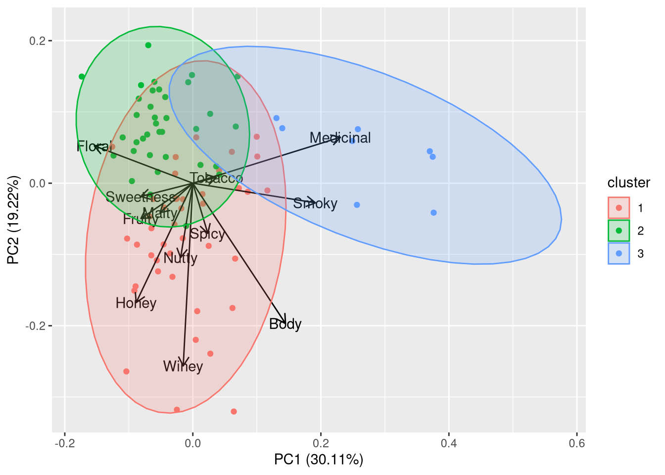
By visualizing the clusters on a biplot, which overlays the original variable vectors onto the PCA plot, we can directly see which behaviors define each group.
Conclusion
Today, we've moved from a simple map of suspects to a strategic analysis of their organization. By applying clustering algorithms like K-Means and Hierarchical Clustering to our PCA-reduced data, we can segment individuals into meaningful behavioral groups. This is not just a data processing step; it is the core of our intelligence gathering. By creating detailed profiles for each cluster, we can distinguish the disorganized rabble from the coordinated, professional crew—and in doing so, we move one giant step closer to unmasking our mastermind.
Key Takeaways:
- Clustering is an unsupervised technique for finding natural groupings in data.
- K-Means Clustering groups data by assigning points to the nearest of K pre-specified centroids in an iterative process.
- The optimal number of clusters (K) can be estimated using the Elbow Method (with inertia) and the Silhouette Score.
- Hierarchical Clustering builds a tree of clusters (a dendrogram) without needing K upfront, allowing us to explore different levels of grouping.
- The most critical step is interpreting the clusters: we analyze the average characteristics of each group to build a narrative profile, or "archetype," which turns raw data into actionable insight.
Preview of the Next Lesson
We have now identified several distinct "crews" operating in the periphery of the "Midnight Seraph" boutique. Our analysis points to one cluster as being particularly suspicious—their behavioral signature is unique and highly coordinated. In our next session, we will zoom in on this primary suspect cluster. We will build a predictive model focused exclusively on this group to decode their internal strategy, quantify the factors driving their actions, and ultimately anticipate their next move. The hunt is reaching its climax.