Predicting Suspect Behavior with Multiple Regression

The Anatomy of a Strategy

At its core, any strategy is about allocating resources (our inputs) to achieve a desired outcome. For our Shadow Crew, let's imagine we've gathered data on several of their past "operations." For each operation, we have data on the resources they deployed and the resulting "Impact Score"—a metric we've devised to measure the operation's success.

Our goal is to find a mathematical relationship between these inputs and the outcome. This is the domain of Multiple Linear Regression (MLR). While simple linear regression models an outcome based on a single predictor, multiple regression allows us to use several predictors simultaneously. It's the perfect tool for understanding a complex system with many moving parts, like a criminal strategy.

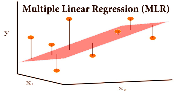
The model assumes that the outcome (Impact Score) is a linear combination of the various strategic inputs. For two predictor variables, say $X_1$ (e.g., Online Disinformation Effort) and $X_2$ (e.g., Financial Anomaly Score), the model tries to find the best-fitting plane through the data points in three-dimensional space.

Let's formalize this.

In our case:

• Y is the n x 1 vector of "Impact Scores" from n past operations.
• X is the n x (k+1) matrix of our k "strategic input" variables for each operation (plus a column of ones for the intercept).
• β is the (k+1) x 1 vector of unknown regression coefficients. These coefficients are what we need to find; they represent the core of the mastermind's strategy.
• ϵ is the n x 1 vector of random errors—the part of the Impact Score our model can't explain.

Cracking the Code: The Normal Equations

How do we find the best values for the coefficients in β? We use the method of Ordinary Least Squares (OLS), which aims to find the coefficient values that minimize the sum of the squared errors (the squared lengths of those vertical lines in the image above).

Given your background, you know that this minimization problem has a beautiful closed-form solution when expressed in matrix algebra. This solution is known as the normal equation.

By applying this formula to the data from our suspect cluster, we can compute the estimated coefficient vector, $\hat{\beta }$. This vector is our first draft of the mastermind's playbook.

Decoding the Playbook: Interpreting the Coefficients

Finding the numbers is only the first step. The real detective work lies in interpreting them. Each coefficient in our $\hat{\beta }$ vector tells a story about the crew's strategy.

A key concept here is that of a partial regression coefficient. In multiple regression, each coefficient's interpretation comes with a crucial caveat: "holding all other variables constant."

This video provides an excellent walkthrough of how to interpret the numbers you'll get from a regression output.

So, if the coefficient for "Online Disinformation Effort" is +5.2, it means that for every one-unit increase in their disinformation campaign, the operation's Impact Score is expected to increase by 5.2 points, assuming their financial activity and recruitment levels remain the same. This allows us to isolate the unique contribution of each strategic lever.

Comparing Apples and Oranges: Standardized vs. Unstandardized Coefficients

This brings us to a critical question: which factor is most important to their strategy? Let's say our predictors are:

• $X_1$: Online Disinformation Effort (measured in "engagement units")
• $X_2$: Financial Anomaly Score (measured in dollars)

A coefficient of +5.2 for $X_1$ and +0.01 for $X_2$ doesn't automatically mean disinformation is more important. The scales are completely different. To compare their relative importance, we need to put them on a common scale. We do this by calculating standardized coefficients.

If the standardized coefficient for disinformation (${\beta }_1$) is 0.65 and for financial anomalies (${\beta }_2$) is 0.30, we can now confidently say that disinformation has more than double the strategic weight in their model of success. This is how we "quantify the factors driving their strategy."

Validating Our Intelligence

Before we can trust our model to predict the crew's next move, we must assess its quality. Is it a reliable tool, or just statistical noise? We look at a few key indicators.

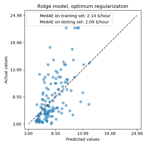
Here are the key questions we need to ask, which are covered in the following video:

1. Does the model work at all? We use the F-statistic to test if our set of predictors, as a whole, explains a significant amount of the variation in the Impact Score.
2. Which factors matter? We use t-tests for each individual coefficient to see if its contribution is statistically significant or if it could just be due to random chance.
3. How much does it explain? The R-squared ($R^2$) value tells us the proportion of the variance in the Impact Score that our model can explain. An $R^2$ of 0.75 means we can account for 75% of why some operations succeed more than others.

Predicting the Next Move

Once we have a validated model, we have a powerful predictive tool. Our final regression equation will look something like this:

Now, if our surveillance picks up chatter indicating the crew is planning an operation with specific levels of disinformation, financial movement, and stealth, we can plug those values into our equation. The result is a quantitative prediction of how impactful their next move will be, allowing us to allocate our own resources proactively.

This is the ultimate goal of our analysis: to move from reacting to the mastermind's actions to anticipating them.

Conclusion

Today, we've taken a significant step from identification to prediction. By focusing our analytical lens on the "Shadow Crew," we've laid the groundwork for building a multiple linear regression model of their strategic behavior. This model is more than just an equation; it's a window into the mind of our adversary.

Key Takeaways:

• Multiple Linear Regression (MLR) allows us to model a single outcome variable using multiple predictor variables.
• The model coefficients ($\beta$) can be estimated using the matrix formula $\hat{\beta }=(X^{T}X{)}^{-1}{X}^{T}Y$.
• Unstandardized coefficients are used for making predictions in the original units of the data.
• Standardized coefficients are used to compare the relative importance of each predictor in the strategy, holding all other factors constant.
• We assess the model's quality using the overall F-test, individual t-tests for each coefficient, and the R-squared value.
• A validated model allows us to predict future outcomes based on the inputs, turning our analysis into actionable intelligence.

Preview of the Next Lesson

We have now developed all the components of our investigation. We used PCA to find the signal in the noise, clustering to identify the key players, and regression to build a predictive model of their strategy. In our final session, we will put it all together. We will synthesize the evidence from all three analyses to construct a comprehensive profile of the mastermind and their operation, leading us to the final gambit to close the case.