Welcome back, Detective. Our last session was a breakthrough. By dissecting the flood of bookings into its constituent streams, we moved beyond mere suspicion to hard evidence. The data confirmed that the anomaly was not a natural surge of interest but a targeted attack on the Aphrodite's Veil website portal. We have found the saboteur's weapon.
However, a good investigation must consider all consequences of a crime. The studio's reputation doesn't just rest on its booking system; it's built on the success of the relationships it helps to foster. This raises a new, more profound question: beyond the sabotage, is there a deeper problem at Aphrodite's Veil? Do the relationships formed under its guidance flourish, or are they unusually fragile?
In this next phase of our investigation, we will pivot from the arrival of clients to the duration of their subsequent relationships. To do this, we need a new set of tools designed to analyze "time-to-event" data. Our objective is to compute and interpret the fundamental metrics of survival analysis—the survival and hazard functions—to determine if, and more importantly when, the risk of a relationship ending begins to accelerate.
A New Line of Inquiry: Time-to-Event Analysis
When we want to understand the lifespan of something—be it a mechanical part, a patient's recovery, or a romantic relationship—we enter the realm of survival analysis. This statistical field is uniquely equipped to handle data about durations.
The video below provides a great high-level introduction to the core ideas. As you watch, pay attention to how the analysis is framed around an "exposure" (like getting married) and an "event" (like getting divorced), and how survival is visualized over time.
Introduction to Survival Analysis [1/8]
This segment from zedstatistics' "Introduction to Survival Analysis" will set the stage for our new investigative tools.
First, watch the introductory explanation of what survival analysis is, including the example of divorce rates. Then, watch the section that explains how to measure and visualize survival time, which introduces the basic form of a Kaplan-Meier curve.
As the video hints, one of the main reasons we need specialized methods is the problem of censoring. In our case, if we follow 10 couples for a year, some might break up (the "event" occurs), but others will still be together when our study ends. We can't just discard these ongoing relationships; they provide the crucial information that they have survived at least until the end of the study. This is known as right-censoring.
The Survival Function: The Probability of Longevity
The first key metric in our new toolkit is the survival function, denoted . It answers a simple but powerful question: What is the probability that a relationship will last longer than a specific amount of time, ?
Formally, if is the random variable representing the time until the event (a breakup), then:
The survival function is always a non-increasing function that starts at (the probability of a relationship lasting longer than time 0 is 100%) and approaches .
The following resource provides a concise definition of the survival function and other key concepts.
What is survival analysis? Examples by hand and in R - Stats and R
This article from the blog 'statsandr' gives a clear and practical introduction to the core functions of survival analysis.
First, read the introduction for a broader context on what survival analysis is and why we need special methods like censoring. Then, focus on the section defining the Survival function.
The Hazard Function: The Instantaneous Risk of Failure
While the survival function tells us about longevity, the hazard function, , gives us a more dynamic view of risk. It represents the instantaneous rate of failure at time , given that the relationship has survived up to time .
Think of it as the "breakup risk" on any given day, for couples who are still together. Unlike a probability, the hazard rate is not bounded by 1; it is a rate.
The hazard function is our primary tool for detecting when risk accelerates. A low, flat hazard function suggests relationships are stable. A hazard function that increases over time indicates a "wear-out" effect, where the risk of a breakup grows as the relationship ages.
The relationship between the survival function and the hazard function is direct: a steep drop in the survival curve corresponds to a high hazard rate.
What is survival analysis? Examples by hand and in R - Stats and R
Let's return to the same article to formally define the hazard function.
Read the section on the Hazard function. Notice the key relationship h(t) = f(t)/S(t), where f(t) is the probability density function of failure times.
Hazard functions can take many shapes, which reveal the underlying nature of the risk. The image below shows four common patterns from the Weibull distribution family.
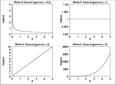
In our investigation, we are looking for evidence of an increasing hazard (), which would suggest a systemic problem causing relationships to become less stable over time.
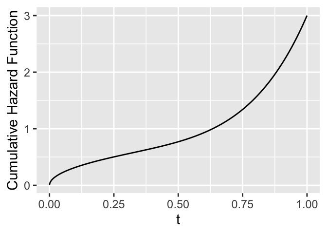
Finally, integrating the hazard function over time gives us the cumulative hazard function, . This represents the total accumulated risk up to time . It's related to the survival function by a simple formula: .
Case File: Analyzing Relationship Durations at Aphrodite's Veil
Now, let's apply these tools. We have obtained a small, anonymized sample of data for 10 client relationships initiated through Aphrodite's Veil. The data records the duration of the relationship in months and whether it ended (event=1) or was still ongoing at the time the data was collected (event=0, i.e., censored).
| Client ID | Duration (months) | Status (1=Ended, 0=Ongoing) |
|---|---|---|
| AV-01 | 3 | 0 (Censored) |
| AV-02 | 5 | 1 (Event) |
| AV-03 | 7 | 1 (Event) |
| AV-04 | 2 | 1 (Event) |
| AV-05 | 18 | 0 (Censored) |
| AV-06 | 16 | 1 (Event) |
| AV-07 | 2 | 1 (Event) |
| AV-08 | 9 | 1 (Event) |
| AV-09 | 16 | 1 (Event) |
| AV-10 | 5 | 0 (Censored) |
To estimate the survival function from this data, we use the Kaplan-Meier estimator. This non-parametric method calculates the survival probability at each point in time an event occurs.
The resource below provides a fantastic, step-by-step guide to calculating the Kaplan-Meier estimate by hand. We will follow this exact procedure for our case data.
What is survival analysis? Examples by hand and in R - Stats and R
This section will guide you through the numerical core of our analysis.
Please read the entire section on Estimation, focusing on the "By hand" calculation. Follow the logic of creating the table step-by-step. This is precisely what you need to do to solve our case.
Let's construct the Kaplan-Meier table for the Aphrodite's Veil data.
- Ordered distinct event times (): 2, 5, 7, 9, 16
- Number of events at each time ():
- At , 2 relationships ended.
- At , 1 relationship ended.
- At , 1 relationship ended.
- At , 1 relationship ended.
- At , 2 relationships ended.
- Number of individuals at risk just before each event time ():
- At , all 10 clients are at risk.
- At , 7 clients are at risk (10 - 2 who ended at t=2 - 1 who was censored at t=3).
- At , 5 clients are at risk (7 - 1 who ended at t=5 - 1 who was censored at t=5).
- At , 4 clients are at risk (5 - 1 who ended at t=7).
- At , 3 clients are at risk (4 - 1 who ended at t=9).
The Kaplan-Meier estimator is the cumulative product:
Here is the final calculation table:
| 2 | 2 | 10 | 0.800 | 0.800 |
| 5 | 1 | 7 | 0.857 | 0.800 * 0.857 = 0.686 |
| 7 | 1 | 5 | 0.800 | 0.686 * 0.800 = 0.549 |
| 9 | 1 | 4 | 0.750 | 0.549 * 0.750 = 0.412 |
| 16 | 2 | 3 | 0.333 | 0.412 * 0.333 = 0.137 |
Interpretation of the Clues:
- Survival Probability: The probability that a relationship from Aphrodite's Veil lasts longer than 7 months is approximately 54.9%.
- Median Survival: The median survival time is the point where . Looking at our table, this occurs between 7 and 9 months. We estimate the median survival time is 9 months. Half of the relationships have ended by the 9-month mark.
- Hazard Shape: By observing the survival curve (which you can sketch from the table), we see it drops by 20% in the first 2 months (from 1.0 to 0.8), but then drops by a larger proportion later on. For instance, at t=16, the conditional probability of failure is , or ~67%, causing the survival probability to plummet from 41.2% to 13.7%. This pattern—steeper declines later in time—suggests an increasing hazard function. The risk of a relationship ending appears to accelerate over time.
Conclusion
Today, we've opened a new front in our investigation, moving from operational sabotage to client outcomes. By employing the tools of survival analysis, we've developed a way to quantify the longevity and risk associated with the relationships formed at Aphrodite's Veil.
Your key takeaways for the case file:
- Survival Analysis is the statistical framework for analyzing time-to-event data, correctly handling censored observations.
- The Survival Function gives the probability of surviving beyond time . We can estimate it from data using the Kaplan-Meier estimator.
- The Hazard Function measures the instantaneous risk of an event at time , given survival up to that point. Its shape (decreasing, constant, or increasing) reveals the dynamics of risk over time.
- The Verdict (Preliminary): The data from our small sample suggests an increasing hazard rate for relationships from Aphrodite's Veil. This implies that the risk of a breakup is not constant but grows as the relationship matures, a potential sign of a systemic issue that warrants further investigation.
Preview of the Next Lesson
Our analysis so far has been non-parametric, meaning we haven't assumed a specific underlying distribution for the relationship durations. However, your background in stochastic processes reminds us that simple, powerful models are often the most revealing. In the previous lesson, we saw how the exponential distribution (with its constant hazard rate) is linked to the Poisson process.
In our next session, we will investigate whether the simple exponential model fits our data. To do this, we'll need to learn how to estimate its rate parameter, , from a dataset that includes the censored observations we've discussed today. This will involve one of the most fundamental techniques in all of statistics: Maximum Likelihood Estimation.