Estimating Attrition with Censored Data using MLE

Welcome back, Detective.

In our last session, we uncovered a disturbing pattern. The Kaplan-Meier analysis of relationship durations from Aphrodite's Veil hinted at an increasing hazard rate—meaning the risk of a relationship ending seems to grow over time. This contradicts the ideal of relationships strengthening with age and points toward a potential systemic flaw in the studio's matchmaking or support process.

However, a good detective never relies on a single piece of evidence. Your background in stochastic processes reminds us that many real-world phenomena, like call arrivals or radioactive decay, can be elegantly described by the exponential distribution, which is defined by a constant event rate. This gives us a competing hypothesis: perhaps the attrition at Aphrodite's Veil is constant, and our previous finding was just an artifact of a small sample.

Today, we will put this simpler theory to the test. Our objective is to estimate a single, constant "attrition rate" for the relationships, assuming they follow an exponential decay pattern. To do this with our incomplete data—which includes those ongoing, "censored" relationships—we must turn to one of the most powerful tools in our arsenal: Maximum Likelihood Estimation (MLE).

The Principle of Maximum Likelihood

Before we tackle the complexity of censored data, let's refresh the core idea of MLE. Given a set of observations, MLE finds the parameter values for a chosen distribution that make observing that specific data most probable.

The video below from StatQuest offers an excellent, intuitive explanation of how MLE is used to find the rate parameter, $λ$ , for an exponential distribution, assuming we have complete data.

Maximum Likelihood for the Exponential Distribution, Clearly Explained!!!

This StatQuest video, "Maximum Likelihood for the Exponential Distribution, Clearly Explained!!!", will serve as our foundation.

Watch the entire video. Pay close attention to these steps: The initial explanation of the exponential distribution and its rate parameter, \lambda. How to construct the likelihood function by multiplying the probabilities of each independent observation. The process of using the log-likelihood and calculus to derive the MLE for \lambda. Finally, see how to apply the formula to data.

The key result for uncensored data is that the MLE for the rate $λ$ is simply the inverse of the sample mean. But what happens when we can't observe all the event times?

Incorporating Censored Data into the Likelihood

Our data contains two types of information, as visualized in the chart below. Some participants have an "Event" (a breakup), for which we know the exact time. Others are "Censored"—we only know they lasted at least as long as their observation time.

This timeline illustrates our data challenge. For participants with a red dot (Event), we have an exact duration. For those with a green dot (Censor), we only have a lower bound on their duration.

To build a likelihood function that uses all this information, we combine two different kinds of probabilities:

For an uncensored observation (a breakup at time $t_{i}$ ), its contribution to the likelihood is the value of the probability density function (PDF) at that time. For an exponential distribution with rate $λ$ , this is $f (t_{i}) = λ e^{- λ t_{i}}$ . This is the "probability" of the event happening in an infinitesimal window around $t_{i}$ .
For a right-censored observation (a relationship is still ongoing at time $t_{i}$ ), we don't know the failure time. The only information we have is that the true duration $T$ is greater than $t_{i}$ . Therefore, its contribution is the probability of this fact, which is the survival function, $S (t_{i}) = P (T > t_{i}) = e^{- λ t_{i}}$ .

The total likelihood is the product of these individual contributions. Let $U$ be the set of uncensored observations and $C$ be the set of censored observations. The likelihood function $L (λ)$ is:

$L (λ) = (\prod_{i \in U} f (t_{i})) (\prod_{j \in C} S (t_{j})) = (\prod_{i \in U} λ e^{- λ t_{i}}) (\prod_{j \in C} e^{- λ t_{j}})$

This elegant construction allows us to use every piece of information we have. The following resource from the University of South Carolina provides a formal walkthrough of this logic.

[PDF] STAT 513 fa 2020 Lec 11 - Censored data and survival analysis

These lecture notes by Karl B. Gregory formally detail the process of building a likelihood function with censored data.

First, review the introduction to understand the formal notation for censored data. Then, read the section on MLE with censored data which explains how the PDF and survival function are combined. Finally, work through the Exercise where this is applied directly to the exponential distribution. Note that the resource estimates the mean lifetime \lambda, whereas we are interested in the rate parameter, which is simply 1/\lambda. The logic is identical.

Deriving the Attrition Rate

By combining the terms in our likelihood function, we get:

$L (λ) = λ^{n_{U}} exp (- λ \sum_{i \in U \cup C} t_{i})$

where $n_{U}$ is the number of uncensored observations (events).

As the StatQuest video showed, it's easier to work with the log-likelihood, $ℓ (λ) = ln (L (λ))$ :

$ℓ (λ) = n_{U} ln (λ) - λ \sum_{i = 1}^{n} t_{i}$

To find the value of $λ$ that maximizes this function, we take the derivative with respect to $λ$ and set it to zero:

$\frac{\partial ℓ}{\partial λ} = \frac{n _{U}}{λ} - \sum_{i = 1}^{n} t_{i} = 0$

Solving for $λ$ gives us our maximum likelihood estimator, $λ^$ :

$λ^= \frac{n _{U}}{\sum _{i = 1}^{n} t _{i}} = \frac{Number of Events (Breakups)}{Total Time Observed (for all clients)}$

This result is wonderfully intuitive. The estimated attrition rate is simply the number of breakups we saw divided by the total "relationship-months" we observed. This properly accounts for the time contributed by the censored relationships. The following resource from Math StackExchange provides another perspective on this derivation and a helpful justification for the method.

Likelihood of censored exponential random variables

This Stack Exchange answer provides a concise derivation and addresses a common point of confusion.

Read the main answer section to see the derivation of the log-likelihood and the resulting MLE for \hat{\lambda}. Then, read the final paragraphs explaining why it's valid to mix probabilities and densities in the likelihood function. This is a subtle but important point that solidifies the theory.

Case File: Calculating the Attrition Rate for Aphrodite's Veil

Let's apply this to our case data from the previous lesson:

Client ID	Duration (months)	Status (1=Ended, 0=Ongoing)
AV-01	3	0 (Censored)
AV-02	5	1 (Event)
AV-03	7	1 (Event)
AV-04	2	1 (Event)
AV-05	18	0 (Censored)
AV-06	16	1 (Event)
AV-07	2	1 (Event)
AV-08	9	1 (Event)
AV-09	16	1 (Event)
AV-10	5	0 (Censored)

Count the number of events ( $n_{U}$ ): There are 7 breakups (events).
Calculate the total time observed ( $\sum t_{i}$ ): 3 + 5 + 7 + 2 + 18 + 16 + 2 + 9 + 16 + 5 = 83 months.

Now, we compute the estimated attrition rate:

$λ^= \frac{7}{83} \approx 0.0843$

Interpretation: Our model estimates a constant attrition rate of approximately 8.4% per month. This implies that for any given month, a relationship has an 8.4% chance of ending, regardless of how long it has already lasted. This also implies a mean relationship lifetime of $1/ λ^\approx 1/0.0843 \approx 11.86$ months.

The Verdict: A Deeper Conspiracy?

We now have two competing pictures of reality: the non-parametric Kaplan-Meier curve from last lesson suggesting an accelerating risk, and a simple exponential model with a constant risk. A visual comparison is telling.

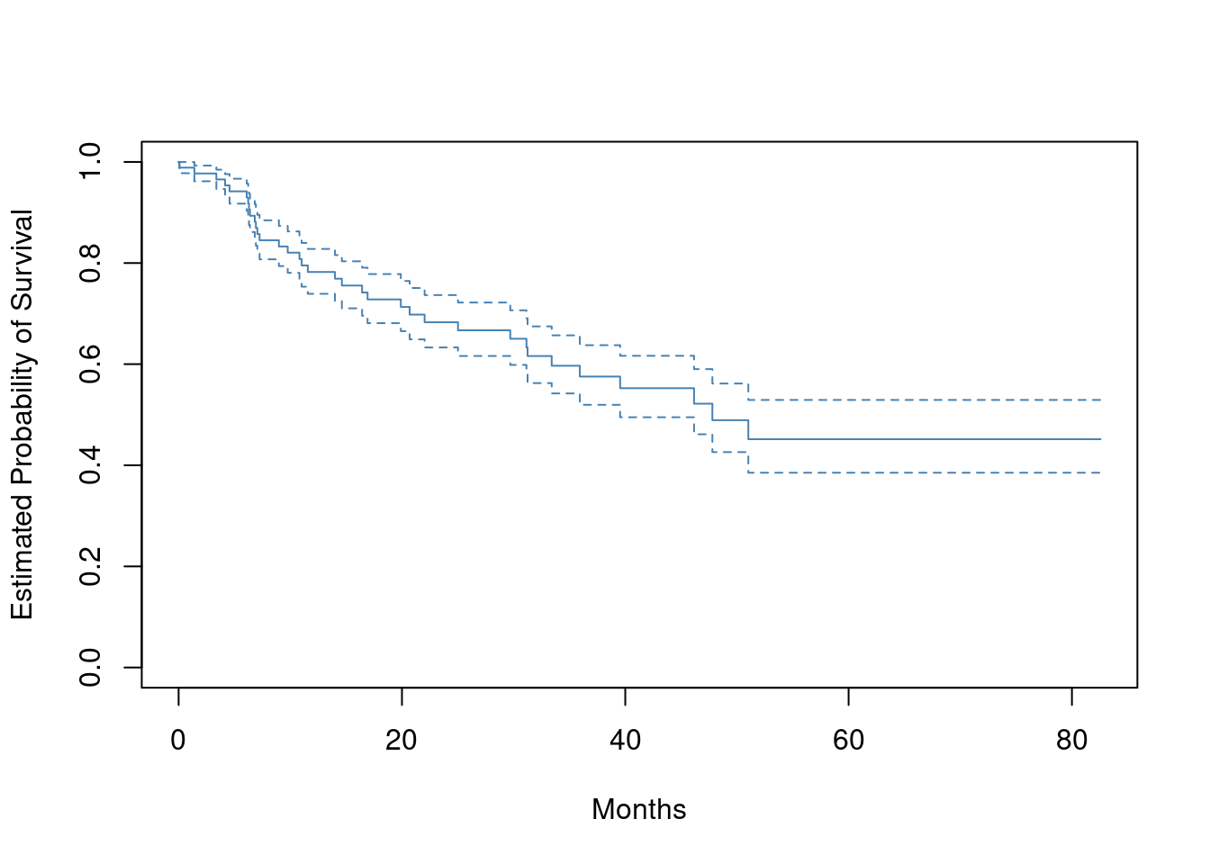
Recall the step-wise Kaplan-Meier curve from our previous analysis. An exponential survival curve, S(t) = e⁻⁰.⁰⁸⁴³ᵗ, would be a smooth, convex curve decaying from 1. It would likely fall faster than the KM curve initially and not as steeply at the end.

When we plot our new exponential survival function over the Kaplan-Meier estimate, we would likely see a discrepancy. The exponential model, with its constant risk, cannot capture the sharp, late-stage drop-offs that our non-parametric analysis hinted at. This poor fit is evidence against the simple "constant attrition" theory and lends more weight to our initial suspicion: something is causing relationships to become more fragile over time.

But there's another layer to this. Our entire analysis hinges on a crucial assumption: uninformative censoring. We assume that the reason a relationship is censored is independent of its outcome. What if that's not true? What if the couples who are still together (censored) are the most dedicated ones, and the couples prone to breaking up have already been filtered out? This would mean our estimate of the attrition rate is biased. The following video explores the dramatic consequences of this assumption being violated.

How to read Kaplan-Meier plots

This video, "How to read Kaplan-Meier plots" from Vinay Prasad's channel, provides a masterclass in critically evaluating survival data.

First, watch the general introduction to reading the plots and the key assumption of uninformative censoring. Then, pay close attention to the case study where the speaker identifies and analyzes an imbalance in censoring, suspecting it is informative. Finally, see how different assumptions about the censored population can drastically change the conclusions.

This critical perspective is essential for a detective. The patterns in the data are only as reliable as the assumptions used to generate them. The possibility of informative censoring opens up a new avenue of inquiry: are the clients who drop out of the study (or remain) systematically different?

Conclusion

Today we wielded the powerful tool of Maximum Likelihood Estimation to handle the challenge of censored data. We formulated a competing theory—that relationship attrition is constant—and derived a precise estimate for this rate.

Your key takeaways for the case file:

Likelihood for Censored Data: The likelihood function for a dataset with right-censored observations is the product of the PDF values for the events and the survival function values for the censored times.
MLE for Exponential Rate: For an exponential distribution with rate $λ$ , the MLE from censored data is $λ^= (number of events) / (total time observed)$ .
Model Comparison: By comparing the fit of our simple exponential model to the non-parametric Kaplan-Meier curve, we found evidence against the constant-rate hypothesis. The initial suspicion of an increasing hazard remains the most likely explanation for the data.
Investigative Caveat: All survival analysis relies on the assumption of uninformative censoring. Any violation of this assumption could fundamentally alter our conclusions.

Preview of the Next Lesson

Our investigation into the operations at Aphrodite's Veil has revealed potential issues in both its booking systems and client relationship outcomes. The plot thickens. We will now turn our attention to another aspect of the business: a competitive lingerie design contest held by the studio. A disgruntled anonymous tip claims the contest was rigged. In our next module, we will begin a new investigation, "The Unfair Advantage," where our first task will be to determine if the winning design's score was statistically plausible or an outrageous outlier. To do this, we will need to master the tools of order statistics.

Recommended resources