Order Statistics: Fairness Benchmarks in Design Contests

Cold Opening: The Unfair Advantage

You receive an anonymous, encrypted email. The sender, claiming to be a former employee at Aphrodite's Veil, is brief and bitter.

They rigged it. The whole "Siren's Silhouette" lingerie design contest. Look at the winner. An unknown. Score of 99.8. Impossible. They didn't even look at all the finalists properly. It was a setup from the start.

The contest was a major PR event for the studio. Twenty finalist designs were chosen, and a panel of judges scored them on a scale of 0 to 100. A score of 99.8 is indeed spectacular. But is it impossibly so? Before we can investigate claims of a fixed process, we must first determine if the outcome itself is a statistical red flag. If scores were assigned fairly and randomly, what would we expect the winning score to be?

This brings us to a new line of inquiry. In this module, "The Unfair Advantage," our first objective is to use order statistics to determine the expected value and variance of the highest and lowest scores in the design contest, establishing a benchmark for fairness.

From a Sample to a Ranked Set

When we have a collection of random observations, like the 20 scores from the judges, we usually assume they are independent and identically distributed (i.i.d.). But what happens when we sort them? The resulting values—the minimum, the second smallest, the median, the maximum—are called order statistics.

Your background in statistics has made you intimately familiar with some of these, like the sample minimum, maximum, and median. These are fundamental to descriptive statistics and non-parametric methods. However, thinking of them as random variables in their own right, each with its own distribution, opens up a powerful new analytical framework.

The video below gives a clear and concise introduction to this idea.

A crucial insight, as Professor Joe Blitzstein from Harvard University points out, is that while the original observations $X_1,...,X_n$ might be independent, the sorted order statistics $Y_1,...,Y_n$ are inherently dependent. If you know the minimum score ($Y_1$) was 80, you immediately know the maximum score ($Y_n$) must be at least 80.

The Anatomy of a Rank

To determine if a score of 99.8 is plausible, we need the probability distribution of the maximum value. Let's build the intuition for the probability density function (PDF) of the k-th order statistic, $Y_k$.

Imagine our number line of scores from 0 to 100. For one specific value, $y$, to be the k-th highest score, three things must happen simultaneously for our sample of $n$ designs:

1. One design must have a score that falls in an infinitesimally small interval around $y$.
2. Exactly $k-1$ other designs must have scores less than $y$.
3. The remaining $n-k$ designs must have scores greater than $y$.

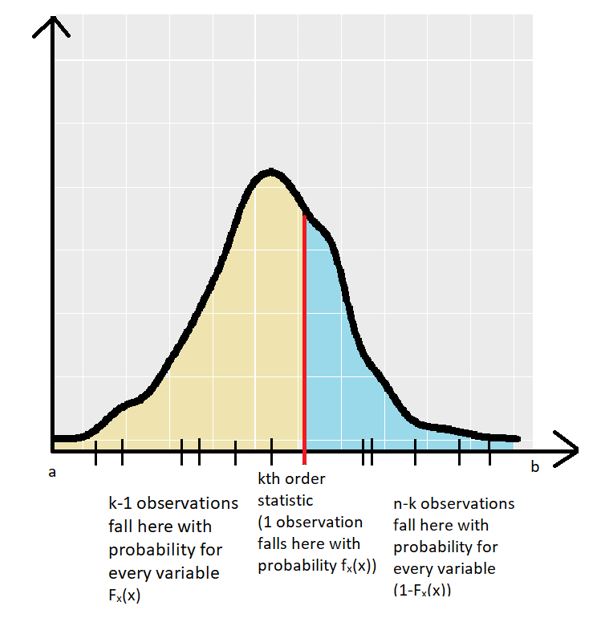
This setup feels remarkably similar to a binomial trial, a concept you're well-versed in. We have $n$ items to place into three bins: "less than y," "at y," and "greater than y." Using a combinatorial argument, we can derive the general formula for the PDF of $Y_k$. The following video walks through this elegant derivation.

This reasoning leads to the general formula for the PDF of the k-th order statistic, $Y_k$, from a continuous distribution with PDF $f(y)$ and CDF $F(y)$:

$f_{Y_k}(y)=\frac{n!}{(k-1)!(n-k)!}[F(y){]}^{k-1}[1-F(y){]}^{n-k}f(y)$

The term $\frac{n!}{(k-1)!(n-k)!}$ is a multinomial coefficient which counts the number of ways to assign the $n$ observations to the three bins.

Establishing a Baseline: The Uniform Judge

To start our investigation, let's form a null hypothesis: The judges are completely unbiased and assign scores purely at random. This is equivalent to modeling the scores as independent draws from a Uniform distribution on the interval [0, 100].

While this model is simplistic, it provides a crucial baseline. If the observed winning score is highly improbable even under this random model, it gives us strong grounds for suspicion.

The uniform distribution makes our math much simpler. For a standard uniform U(0,1), the PDF is $f(y)=1$ and the CDF is $F(y)=y$ for $y\in [0,1]$. Plugging this into our general formula gives the PDF for the k-th order statistic from a U(0,1) sample:

$f_{Y_k}(y)=\frac{n!}{(k-1)!(n-k)!}{y}^{k-1}(1-y{)}^{n-k}$

This is the PDF of a Beta distribution with parameters $\alpha =k$ and $\beta =n-k+1$. This connection is a cornerstone of order statistics and provides us with ready-made formulas for the expected value and variance.

The following resource formally derives these results.

Case File: Calculating the Benchmark

Now, let's apply these tools to the "Siren's Silhouette" contest.

• Number of finalists, $n=20$.
• Scores are on a scale of [0, 100].

Our formulas are for a U(0,1) distribution. We can scale the results using the properties of expectation and variance. If $Y$ is a score on [0,1] and $Z$ is a score on [0, 100], then $Z=100Y$.
Therefore, $E[Z]=100\cdot E[Y]$ and $Var(Z)=100^2\cdot Var(Y)$.

1. The Highest Score (The Winner)

We are interested in the maximum score, which is the n-th order statistic, $Y_{20}$. Here, $k=n=20$.

• Expected Value:
  $E[Y_{20}]=\frac{20}{20+1}=\frac{20}{21}\approx 0.9524$
  Scaling to our [0, 100] range:
  $E[\text{Highest Score}]=100\times 0.9524=95.24$
  So, under a purely random judging model, we'd expect the winning score to be around 95.24.

• Variance:
  $Var(Y_{20})=\frac{20(20-20+1)}{(20+1{)}^2(20+2)}=\frac{20}{21^2\times 22}=\frac{20}{441\times 22}=\frac{20}{9702}\approx 0.00206$
  Scaling to our [0, 100] range:
  $Var(\text{Highest Score})=100^2\times 0.00206=10000\times 0.00206=20.6$
  The standard deviation is $\sqrt{20.6}\approx 4.54$.

2. The Lowest Score (The Unluckiest Finalist)

For completeness, let's also calculate the expected lowest score, $Y_1$. Here, $k=1$.

• Expected Value:
  $E[Y_1]=\frac{1}{20+1}=\frac{1}{21}\approx 0.0476$
  Scaling to our [0, 100] range:
  $E[\text{Lowest Score}]=100\times 0.0476=4.76$

• Variance:
  $Var(Y_1)=\frac{1(20-1+1)}{(20+1{)}^2(20+2)}=\frac{20}{21^2\times 22}=\frac{20}{9702}\approx 0.00206$
  Notice the variance of the minimum is the same as the variance of the maximum. This is due to the symmetry of the uniform distribution.
  $Var(\text{Lowest Score})=100^2\times 0.00206=20.6$
  The standard deviation is also $\approx 4.54$.

Initial Verdict

The anonymous tip claimed the winning score of 99.8 was "impossible." Our analysis provides a way to quantify this.
The expected highest score was 95.24, with a standard deviation of 4.54. The observed score of 99.8 is:
$\frac{99.8-95.24}{4.54}\approx \frac{4.56}{4.54}\approx 1.004$
The winning score is almost exactly one standard deviation above the mean. In a roughly bell-shaped distribution (which the Beta distribution for the maximum often is), this is not a rare event at all (roughly the 84th percentile).

Based on this first pass, the score itself is not the smoking gun the tipster suggested. It's high, but plausible. Perhaps our assumption of a purely random Uniform distribution is wrong. Maybe talented designers consistently produce high scores, shifting the whole distribution upwards. Or perhaps, as the tipster hinted, the process was flawed.

Conclusion

In this lesson, we opened the case file on "The Unfair Advantage" by establishing a statistical benchmark for fairness. We've seen how to take a seemingly simple concept—ranking—and treat it with the full rigor of probability theory.

Your key takeaways from this investigation:

• Order Statistics: The sorted values of a random sample, $Y_1,...,Y_n$, are themselves random variables with their own distributions.
• PDF of the k-th Order Statistic: We can derive a general formula for this PDF using a combinatorial argument, which for a U(0,1) sample simplifies to a Beta distribution.
• Expected Value and Variance: For a sample of size $n$ from U(0,1), the k-th order statistic $Y_k$ has $E[Y_k]=k/(n+1)$ and $Var(Y_k)=k(n-k+1)/((n+1{)}^2(n+2))$.
• Case Status: A preliminary analysis shows the winning score of 99.8 is only one standard deviation above what would be expected under a purely random judging model. This leads us to question the tipster's claim, or more likely, our initial model.

Preview of the Next Lesson

Our initial analysis assumed all 20 designs were judged simultaneously. But the tipster's email contained another cryptic line: "They didn't even look at all the finalists properly." This suggests a sequential process. What if the judges stopped early? This introduces a new question: if you are looking for the single best candidate in a sequence, when should you stop looking and make your choice?

In our next session, we will investigate this possibility by exploring the famous "secretary problem" and the principles of optimal stopping. We will see if the contest's procedure itself could have been designed to favor an early candidate.