Observer-Based State Verification

The Simulation Strategy

To verify our observer, we need to compare its estimates to the "ground truth." Since we don't have a physical system on hand, we will simulate one. Our strategy involves four main steps:

1. Simulate the "True" System: We'll define a plant model in MATLAB and simulate its response to a given input and initial condition. This will generate the true state trajectory $x(t)$ and the true measured output $y(t)$.
2. Design the Observer: We'll choose desired pole locations for the observer (making them faster than the plant's dynamics) and calculate the observer gain matrix $L$.
3. Simulate the Observer: We'll build the observer's state-space model using the equation above. Then, we'll feed it the input $u(t)$ and output $y(t)$ from our "true" system simulation and run a second simulation to get the estimated state trajectory $\hat{x}(t)$.
4. Compare and Verify: We will plot both $x(t)$ and $\hat{x}(t)$ on the same graph to visually inspect the convergence.

The following video provides a complete, practical walkthrough of this entire process in MATLAB. We will use it as our guide for this lesson.

Step 1 & 2: Simulating the Plant and Designing the Observer

First, we need our "ground truth" data. The video uses a double mass-spring-damper system, which is a great general example. The process involves defining the system matrices $A,B,C,D$, specifying an input signal and initial conditions, and using MATLAB's lsim command to generate the true state and output data.

Simultaneously, we'll design our observer by selecting desired pole locations and using the place command to find the gain $L$. As we've learned, we need to use the duality principle here, applying place to the transposed system matrices (A' and C').

Let's watch how this is done.

After completing these steps, you have:

• The true state history, x_true.
• The true output history, y_true.
• A calculated observer gain matrix, L.

Step 3: Building and Simulating the Observer

Now for the main event. We will construct the observer as a separate state-space system in MATLAB. Recall our observer state equation:

$\dot{\hat{x}}=(A-LC)\hat{x}+\left[\begin{array}{cc}B& L\end{array}\right]\left[\begin{array}{c}u\\ y\end{array}\right]$

This equation tells us exactly how to build the observer's system matrices:

• A_obs = A - L*C
• B_obs = [B, L]
• C_obs = eye(n) (where n is the number of states, since we want the output to be the full state estimate)
• D_obs = zeros(n, m+p) (where m is #inputs, p is #outputs)

The most important part is correctly defining the input for the observer simulation. The term $\left[\begin{array}{c}u\\ y\end{array}\right]$ shows that the observer is driven by both the control input and the measured output of the plant. In MATLAB, this means we need to create a matrix where the first row(s) are the control input u and the next row(s) are the measured output y_true.

We also need to give the observer its own initial condition, x0_observer. To see the convergence happen, it's essential to choose an initial condition that is different from the true system's initial condition. A common choice is to start the observer at zero, x0_observer = [0; 0; 0; 0].

Now, let's see how to implement this final simulation step.

Step 4: Visual Verification

The final step is to plot the results. By plotting the $i$-th true state $x_i(t)$ and the $i$-th estimated state ${\hat{x}}_i(t)$ on the same axes for each state, we can visually confirm the performance of our observer.

You should see something like this:

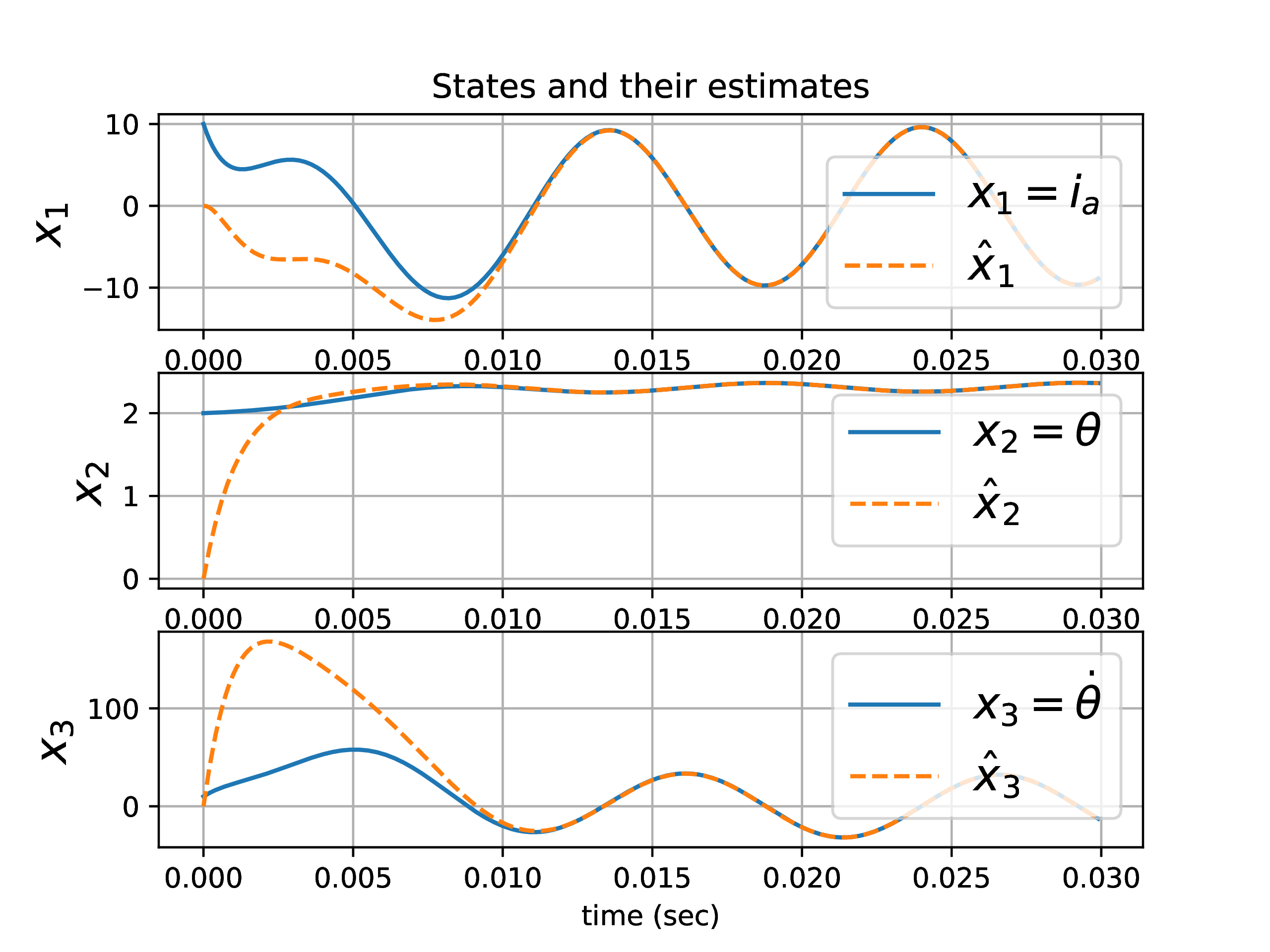
As seen in the video and the image above, the estimated states start from their own initial condition (zero in this case) and, after a brief transient period, converge to and track the true states. The speed of this convergence is dictated by the observer poles we chose in Step 2. If the estimates converge too slowly, you can move the observer poles further into the left-half plane.

The same procedure you've just learned for the mass-spring-damper system applies directly to any LTI system, including your rotary inverted pendulum project. The CTMS page on the inverted pendulum provides MATLAB code that follows a similar logic.

Conclusion

In this lesson, you learned the complete practical workflow for simulating a state observer to verify its performance. This process of simulating a "true" plant and a separate observer is fundamental to testing and validating your designs before deploying them on actual hardware.

Key Takeaways:

• To verify an observer, you simulate a "true" plant to generate $x(t)$ and $y(t)$.
• The observer is constructed as its own state-space system with matrices $A_{obs}=A-LC$ and $B_{obs}=[B,L]$.
• The observer system is driven by a combined input signal composed of the plant's input $u(t)$ and its output $y(t)$.
• By starting the observer from a different initial condition and plotting its states against the true states, you can visually confirm that the estimation error converges to zero at the rate determined by your chosen observer poles.

Preview of the Next Lesson:
We have successfully designed a controller (gain $K$) and an observer (gain $L$). Now it's time to put them together. The next lesson introduces the Separation Principle, a cornerstone of modern control theory. It states that we can design the state feedback controller and the state observer independently and then combine them, and the resulting closed-loop system will be stable. We will see how to implement the control law using our estimated states ($u=-K\hat{x}$) and analyze the properties of the complete observer-based control system.