Observer-Based State Feedback Control: Dynamic Equations

The Structure of an Observer-Based Controller

Let's start by visualizing how all the pieces fit together. The controller is no longer just a static gain; it's a dynamic system that incorporates the observer.

The system consists of three interconnected parts:

1. The Plant: The actual system we want to control.
   $\dot{x}=Ax+Bu$
   $y=Cx$
2. The State Observer: Our real-time model that estimates the plant's state.
   $\dot{\hat{x}}=A\hat{x}+Bu+L(y-C\hat{x})$
3. The Control Law: The feedback rule, now using the estimated state.
   $u=-K\hat{x}+r$
   (where $r$ is an external reference input, which we'll set to 0 for stabilization problems).

The following block diagram shows how these components are interconnected. The plant is the "true system," while the observer and feedback gain $K$ together form the controller (or compensator).

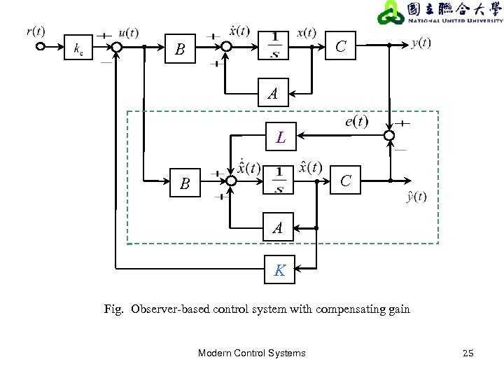
Our task is to take these separate equations and derive a single state-space model that describes the dynamics of this entire setup.

Deriving the Combined System Dynamics

To analyze the complete system, we need a state vector that describes it fully. Since the plant has $n$ states ($x$) and the observer also has $n$ states ($\hat{x}$), the combined system will have $2n$ states.

While we could use $\left[\begin{array}{c}x\\ \hat{x}\end{array}\right]$ as our state vector, a more insightful choice is to use the plant's state $x$ and the estimation error $\tilde{x}=x-\hat{x}$. This choice elegantly separates the system's dynamics, as we will soon see.

Let's derive the differential equations for $x$ and $\tilde{x}$.

1. Dynamics of the Plant State, $x$:
We start with the plant equation and substitute the control law:
$\dot{x}=Ax+Bu=Ax+B(-K\hat{x})$
Now, we replace $\hat{x}$ using our definition of the error, $\hat{x}=x-\tilde{x}$:
$\dot{x}=Ax-BK(x-\tilde{x})$
$\dot{x}=(A-BK)x+BK\tilde{x}$
This first equation tells us something interesting: the dynamics of the true state $x$ behave like the pole-placed system ($A-BK$), but are influenced by a term proportional to the estimation error $\tilde{x}$.

2. Dynamics of the Estimation Error, $\tilde{x}$:
We derived this in a previous lesson, but it's crucial to see it again in this context.
$\dot{\tilde{x}}=\dot{x}-\dot{\hat{x}}$
Substitute the expressions for $\dot{x}$ and $\dot{\hat{x}}$:
$\dot{\tilde{x}}=(Ax+Bu)-(A\hat{x}+Bu+L(y-C\hat{x}))$
The $Bu$ terms cancel out. We also substitute $y=Cx$:
$\dot{\tilde{x}}=A(x-\hat{x})-L(Cx-C\hat{x})$
Recognizing that $\tilde{x}=x-\hat{x}$, this simplifies beautifully:
$\dot{\tilde{x}}=A\tilde{x}-LC\tilde{x}=(A-LC)\tilde{x}$
This second equation is remarkable. It shows that the estimation error dynamics depend only on the observer's design ($A-LC$). They are completely independent of the plant's state $x$ and the control law $K$.

For a rigorous walkthrough of this derivation, the following notes from MIT OpenCourseWare are an excellent resource.

The Complete State-Space Model

Now we can assemble our two derived equations into a single state-space representation for the entire closed-loop system. Using the state vector $\left[\begin{array}{c}x\\ \tilde{x}\end{array}\right]$ and including the reference input $r$, we get:

This is the central result of today's lesson. This $2n\times 2n$ matrix equation is the complete dynamic model of the plant controlled by an observer-based state feedback system.

The most important feature of this system matrix is its block upper-triangular structure, indicated by the zero matrix in the lower-left block. This structure has a profound implication: the eigenvalues of a block-triangular matrix are the eigenvalues of its diagonal blocks.

This means the set of $2n$ poles of the complete system is simply the union of:

• The eigenvalues of $(A-BK)$ (the $n$ desired controller poles).
• The eigenvalues of $(A-LC)$ (the $n$ desired observer poles).

This convenient result, which we will formally name the Separation Principle in the next lesson, is one of the most powerful ideas in modern control theory. It means you can design your controller and your observer independently, and when you connect them, the poles of the overall system will be exactly where you intended them to be.

Application to the Inverted Pendulum

This structure isn't just a theoretical curiosity; it's exactly what you would implement in practice. The following resource shows how this exact formulation is used for the observer-based control of an inverted pendulum.

The Controller as a Dynamic System

There's one more useful way to look at our observer-based controller. Let's think of the controller as a black box that takes the plant's output $y$ as its input and produces the control signal $u$ as its output. What are the dynamics of this box?

Let's rearrange the observer and control law equations:

1. Observer: $\dot{\hat{x}}=A\hat{x}+Bu+L(y-C\hat{x})$
2. Control Law: $u=-K\hat{x}$

Substitute the control law into the observer equation:
$\dot{\hat{x}}=A\hat{x}+B(-K\hat{x})+Ly-LC\hat{x}$
$\dot{\hat{x}}=(A-BK-LC)\hat{x}+(L)y$

The output of our controller box is $u=(-K)\hat{x}$.

We can now write this in a standard state-space format for the controller, where $\hat{x}$ is the controller's state:

• State Equation: $\dot{\hat{x}}=A_c\hat{x}+B_{c}y$
• Output Equation: $u=C_c\hat{x}+D_{c}y$

By comparing terms, we find the controller's matrices:

• $A_c=A-BK-LC$
• $B_c=L$
• $C_c=-K$
• $D_c=0$

This shows that an observer-based state feedback controller is itself a linear time-invariant (LTI) system of order $n$. This is the "compensator" that you would implement in a control system's hardware or software.

Conclusion

In this lesson, we successfully bridged the gap between state feedback design and state estimation. By using the estimated state $\hat{x}$ in our control law, we were able to formulate the complete dynamic equations for the entire observer-controller-plant system.

Key Takeaways:

• An observer-based controller uses the control law $u=-K\hat{x}$.
• The complete closed-loop system has $2n$ states, which can be represented by the plant state $x$ and the estimation error $\tilde{x}$.
• The system's dynamics are described by a block upper-triangular matrix: $$\left[\begin{array}{cc}A-BK& BK\\ 0& A-LC\end{array}\right]$$
• This structure implies that the closed-loop poles are the union of the controller poles (from $A-BK$) and the observer poles (from $A-LC$).
• The controller itself can be modeled as an $n$-th order LTI system with input $y$ and output $u$.

Preview of the Next Lesson:
The beautiful result we discovered today—that the controller and observer designs don't interfere with each other's pole locations—is called the Separation Principle. In our next lesson, we will formally discuss this principle and its profound implications for control system design. We will explore why this separation works and what it means for the practical process of designing and implementing complex controllers.