Infinite-Horizon LQR for Optimal State Feedback

Hello! Welcome to the first lesson of our new module on optimal control.

In our last module, we mastered the pole placement technique, culminating in simulating a full observer-controller system. We saw that while pole placement gives us complete control over the system's dynamics, it leaves us with a critical question: where should we place the poles for the "best" performance? This choice can feel arbitrary and often requires a lot of trial and error.

This lesson introduces a more systematic and powerful approach: the Linear Quadratic Regulator (LQR). Instead of choosing pole locations, LQR allows us to define what "optimal" performance means through a cost function. The LQR algorithm then calculates the feedback gain matrix K that is optimal for that definition. Our goal today is to understand how to set up, or formulate, the LQR problem by defining this cost function.

1. From Pole Placement to Optimal Control

First, it's important to understand that LQR is not a completely new type of controller in terms of its structure. Like pole placement, it results in a full-state feedback law:

$u = - K x$

The fundamental difference lies in how we determine the gain matrix $K$ .

Pole Placement: We decide on specific closed-loop pole locations to dictate the response (e.g., settling time, damping) and solve for the unique $K$ that achieves this.
LQR: We define a cost function that mathematically describes the trade-off between system performance (how well the states are regulated) and the amount of control effort used. LQR then finds the optimal $K$ that minimizes this cost.

This shift in perspective from "placing poles" to "defining performance" is a core concept in modern control theory.

The following video provides an excellent introduction to LQR, contrasting it with pole placement and introducing the idea of optimality through a very intuitive analogy.

What Is Linear Quadratic Regulator (LQR) Optimal Control? | State Space, Part 4

Watch this video from MATLAB to understand the 'why' behind LQR. It frames the problem and uses a great analogy to explain what 'optimal' means in control design.

Please watch the first 5 minutes and 17 seconds (0:00 - 5:17). Pay close attention to the comparison with pole placement and the 'commuting to work' analogy, which perfectly explains the role of a cost function.

2. The LQR Cost Function: Defining "Optimal"

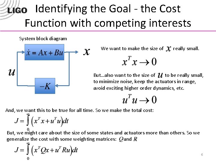
As the video explained, "optimal" is only meaningful relative to a specific goal. In LQR, we codify this goal into a cost function, usually denoted by $J$ . For the infinite-horizon problem (meaning we care about the system's behavior over all future time), the cost function for a continuous-time system is:

$J = \int_{0}^{\infty} (x^{T} (t) Q x (t) + u^{T} (t) R u (t)) d t$

Let's break this down. The LQR controller's objective is to find a control law $u (t)$ that minimizes this total cost $J$ . The cost is composed of two parts integrated over time:

Identifying the Goal - The Cost Function with Competing Interests — This diagram shows the standard state feedback structure and highlights the two components of the LQR cost function: the state cost ($x^TQx$) and the control cost ($u^TRu$).

The State Cost: $x^{T} (t) Q x (t)$

This term penalizes the system for having states that are not zero. Since our goal is to regulate the system to its equilibrium point ( $x = 0$ ), any deviation from zero contributes to the cost.

$x^{T} (t) x (t)$ : This is the squared Euclidean norm of the state vector, $\sum x_{i}^{2} (t)$ . It's a measure of the total "size" or error of the state vector at time $t$ . We square it to ensure the penalty is always positive.
The $Q$ matrix: This is the state weighting matrix. It's a symmetric, positive semi-definite matrix that allows us to specify the relative importance of each state.
- For an $n$ -state system, $Q$ is an $n \times n$ matrix.
- Typically, we choose $Q$ to be a diagonal matrix: $Q = q_{1} 0 ⋮ 0 0 q_{2} ⋮ 0 \dots \dots ⋱ \dots 00 ⋮ q_{n}$
- A large value for a diagonal element $q_{i}$ means we are placing a high penalty on the corresponding state $x_{i}$ being non-zero. The controller will work harder to make that specific state go to zero quickly.

The Control Cost: $u^{T} (t) R u (t)$

This term penalizes the use of control effort. Actuators consume energy, have physical limits, and experience wear and tear. This term represents that "cost."

$u^{T} (t) u (t)$ : Similar to the state cost, this is the squared norm of the control input vector, $\sum u_{j}^{2} (t)$ .
The $R$ matrix: This is the control weighting matrix. It's a symmetric, positive definite matrix that allows us to specify the cost of using each actuator.
- For a system with $m$ inputs, $R$ is an $m \times m$ matrix.
- If $R$ is diagonal, a large value for a diagonal element $r_{j}$ means the corresponding control input $u_{j}$ is "expensive," and the controller will try to use it sparingly.

3. The Performance vs. Effort Trade-off

The essence of designing an LQR controller is choosing the $Q$ and $R$ matrices to balance the trade-off between performance and effort.

Aggressive Control: If you make the elements of $Q$ large relative to the elements of $R$ (high $Q / R$ ratio), you are saying that state errors are very costly and control effort is cheap. The resulting controller will be aggressive, driving the states to zero quickly, but potentially using large control signals.
Conservative Control: If you make the elements of $R$ large relative to the elements of $Q$ (low $Q / R$ ratio), you are saying that control effort is expensive. The controller will be more conservative, using smaller control signals, which will likely result in a slower system response.

The following videos explain these concepts in a very practical way, using the inverted pendulum as an example that should be very relevant to your own project.

What Is Linear Quadratic Regulator (LQR) Optimal Control? | State Space, Part 4

Let's return to the MATLAB video to see a detailed breakdown of the cost function's components.

Please watch from 5:17 to 9:56. This section delves into the mathematical structure of the cost function, explaining the roles of Q and R in detail.

Linear Quadratic Regulator (LQR) Control for the Inverted Pendulum on a Cart [Control Bootcamp]

This video by Steve Brunton provides another excellent explanation, specifically linking the tuning of Q and R to the performance of an inverted pendulum.

Please watch from 1:55 to 5:26. Focus on how he explains the cost function and provides a concrete example of choosing Q matrix values to prioritize stabilizing the pendulum's angle.

Test your understanding!

For your rotary inverted pendulum project, let the state vector be $x = [α, α ˙, θ, θ ˙]^{T}$ , where $α$ is the arm angle and $θ$ is the pendulum angle. The input $u$ is the motor torque. Your primary goal is to keep the pendulum upright ( $θ \approx 0$ ) and stationary ( $θ ˙ \approx 0$ ), and you are less concerned about the arm's final angle or how much energy is used.

How would you choose the relative values in your diagonal $Q$ and $R$ matrices to reflect this priority?

Show answer

To prioritize stabilizing the pendulum angle $θ$ and its velocity $θ ˙$ , you would set the corresponding diagonal elements in the $Q$ matrix to be much larger than the elements for the arm angle $α$ and its velocity $α ˙$ .

For example, you might choose something like:

Q = 1000010000100000050

Here, the penalties for deviations in $θ$ and $θ ˙$ are significantly higher than for $α$ and $α ˙$ .

Since the problem states that you are less concerned about energy usage, you would choose a relatively small value for the $R$ matrix (which is a 1x1 scalar in this case). A small $R$ , like $R = [0.01]$ , tells the controller that control effort is "cheap," allowing it to use aggressive torque commands to stabilize the pendulum.

4. The Formal LQR Problem Statement

We can now formally state the infinite-horizon LQR problem.

Given a linear time-invariant (LTI) system:
$x ˙ (t) = A x (t) + B u (t)$
The goal is to find the constant state-feedback gain matrix $K$ for the control law $u (t) = - K x (t)$ that minimizes the cost function:
$J = \int_{0}^{\infty} (x^{T} (t) Q x (t) + u^{T} (t) R u (t)) d t$
where $Q$ is a positive semi-definite matrix and $R$ is a positive definite matrix.

For digital control implementation, which you'll use in MATLAB, the problem is formulated in discrete-time. The system is $x_{k + 1} = A x_{k} + B u_{k}$ , and the cost function becomes a summation instead of an integral:
$J = \sum_{k = 0}^{\infty} (x_{k}^{T} Q x_{k} + u_{k}^{T} R u_{k})$

The underlying principle is identical: find the gain $K$ that minimizes the total accumulated cost.

Conclusion

In this lesson, you have learned how to formulate the LQR optimal control problem. You've moved beyond the pole-placement mindset of choosing system poles to the LQR mindset of defining performance through a cost function.

Key Takeaways:

LQR finds an optimal gain matrix $K$ by minimizing a quadratic cost function $J$ .
The cost function $J$ quantifies a trade-off between state regulation (penalized by $Q$ ) and control effort (penalized by $R$ ).
The designer's role is to select the weighting matrices $Q$ and $R$ to reflect the desired system behavior and physical constraints. A high $Q / R$ ratio leads to an aggressive response, while a low ratio results in a more conservative one.

Preview of the Next Lesson:
Now that we know how to formulate the problem, the natural next question is: how do we solve it? In the next lesson, we will see how to calculate the optimal feedback gain matrix $K$ . We will introduce the Algebraic Riccati Equation (ARE), the cornerstone of the LQR solution, and see how to use practical tools like the lqr command in MATLAB to find $K$ effortlessly.

Recommended resources