Observer-Controller System Implementation and Simulation

1. The Architecture of an Observer-Based Controller

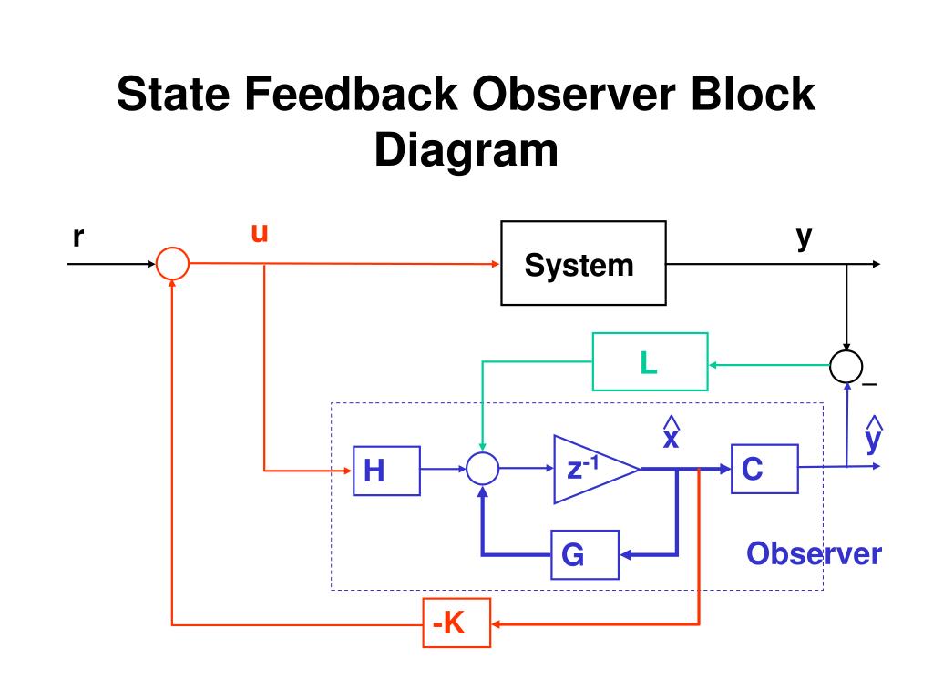
Before we write any code, let's visualize how the components fit together. The controller is no longer using the true state $x$ for feedback. Instead, it relies entirely on the observer's estimate, $\hat{x}$.

The signal flow is as follows:

1. The observer takes the system's control input $u$ and measured output $y$ as its inputs.
2. It continuously computes the state estimate, $\hat{x}$.
3. The control law is now calculated using this estimate: $u=-K\hat{x}$.
4. This control input $u$ is then applied to the actual system (the "plant").

This closed-loop structure is depicted in the block diagram below.

2. Building the Combined System for Simulation

To simulate this entire system, we need to describe it with a single set of state-space equations. The most intuitive way to do this is to create an augmented state vector that includes both the plant's true states $x$ and the observer's estimated states $\hat{x}$.

Let our new augmented state vector be $z=\left[\begin{array}{c}x\\ \hat{x}\end{array}\right]$. This vector has $2n$ states, where $n$ is the number of states in our original system.

Let's derive the state equations for this augmented system.

1. Plant dynamics: The plant's state equation is $\dot{x}=Ax+Bu$. Since the control law is $u=-K\hat{x}$, we can substitute it in:
   $\dot{x}=Ax+B(-K\hat{x})=Ax-BK\hat{x}$

2. Observer dynamics: The observer's state equation is $\dot{\hat{x}}=A\hat{x}+Bu+L(y-\hat{y})$. We can substitute $y=Cx$, $\hat{y}=C\hat{x}$, and $u=-K\hat{x}$:
   $\dot{\hat{x}}=A\hat{x}+B(-K\hat{x})+L(Cx-C\hat{x})$
   Rearranging this by grouping terms with $x$ and $\hat{x}$ gives:
   $\dot{\hat{x}}=(LC)x+(A-BK-LC)\hat{x}$

Now, we can combine these two equations into a single matrix equation for our augmented state vector $z$:

This equation, $\dot{z}=A_{cl}z$, describes the complete, closed-loop system dynamics under state-estimate feedback. This is the model we will implement and simulate.

For a detailed walkthrough of forming this combined system, especially for the inverted pendulum example, the following resource is excellent.

3. Step-by-Step MATLAB Implementation

Let's outline the process for simulating the system's response to an initial perturbation. This is the standard way to verify that both the controller and the observer are working as designed. We'll assume you have your system matrices A, B, C, and have already designed your controller gain K and observer gain L.

Step 1: Define the Augmented System
First, construct the closed-loop matrix A_cl in MATLAB.

% A, B, C, K, L are assumed to be defined
n = size(A, 1); % Number of states

A_cl = [ A,      -B*K;
         L*C,    A - B*K - L*C ];

Step 2: Define Outputs for Plotting
We want to be able to plot both the true states $x$ and the estimated states $\hat{x}$. We can define an augmented output matrix C_cl that selects all $2n$ states.

C_cl = eye(2*n);
D_cl = zeros(2*n, size(B,2)); % Assuming D=0 and no external input

Step 3: Create the State-Space Object
Now, create a single ss object representing the entire system.

sys_cl = ss(A_cl, [], C_cl, []); % No B or D matrix since we'll use initial conditions

The empty brackets [] for the B and D matrices signify that we are simulating a system with no external input, responding only to initial conditions.

Step 4: Set Initial Conditions
This is the most important step for testing the observer. We must give the plant and the observer different initial conditions to see if the observer can converge. A common practice is to give the plant a non-zero initial state and start the observer at zero, simulating a scenario where the observer is turned on with no prior knowledge.

x0 = [0.1; 0; 0; 0];         % Example: Initial 10cm position error for the plant
x_hat0 = [0; 0; 0; 0];        % Observer starts from zero
z0 = [x0; x_hat0];            % Combined initial state vector

Step 5: Simulate and Plot
Use MATLAB's initial command to simulate the response and then plot the results.

t = 0:0.01:5;                % Time vector for simulation
[z, t] = initial(sys_cl, z0, t);

% Extract true and estimated states
x = z(:, 1:n);
x_hat = z(:, n+1:2*n);

% Plotting (example for state 1)
figure;
plot(t, x(:,1), 'b-', 'LineWidth', 2);
hold on;
plot(t, x_hat(:,1), 'r--', 'LineWidth', 2);
grid on;
title('State 1: True vs. Estimated');
xlabel('Time (s)');
ylabel('State value');
legend('True State (x1)', 'Estimated State (x1_hat)');

You would repeat the plotting for all states to verify convergence for each one.

4. A Practical Simulation Walkthrough

The following video provides a great walkthrough of simulating an observer-based system in MATLAB. It uses a slightly different, but very powerful, method involving an ODE solver (ode45). This approach is more general as it can also be used for nonlinear systems. The core principles of setting up the state derivatives remain the same.

Watching this will give you a concrete feel for how these simulations are coded and what the results should look like.

Conclusion

Today, you've learned how to take a designed controller and observer and bring them together into a single, functional, and simulatable system. This is the final step in validating a pole-placement-based control design.

Key Takeaways:

• An observer-based controller uses the state estimate $\hat{x}$ for feedback, with the control law $u=-K\hat{x}$.
• To simulate the complete system, we create an augmented state-space model with state vector $z=[x;\hat{x}]$.
• The system matrix for this combined model is $A_{cl}=\left[\begin{array}{cc}A& -BK\\ LC& A-BK-LC\end{array}\right]$.
• Verifying observer performance requires simulating with different initial conditions for the plant ($x_0$) and the observer (${\hat{x}}_0$).
• The goal is to plot the true vs. estimated states and confirm that the estimation error converges to zero while the overall system remains stable.

Preview of the Next Module:
We have now fully mastered the pole placement design technique. However, you might have noticed that choosing "good" pole locations can be somewhat arbitrary. It requires experience and iteration. What if there were a more systematic method to design a controller that is "optimal" according to some performance criteria?

In our next module, we will begin exploring just that with the Linear Quadratic Regulator (LQR). LQR allows us to find an optimal controller gain $K$ by balancing state regulation against control effort, providing a powerful and elegant alternative to pole placement.