Tuning LQR Weighting Matrices (Q and R)

1. It's All About the Ratio

Before diving into tuning, it's essential to grasp one key concept: in the LQR cost function, it's the ratio of the weights in $Q$ and $R$ that matters, not their absolute values.

Consider the cost function:
$J={\int }_0^{\infty }\left(x^{T}Qx+u^{T}Ru\right)dt$

If we multiply both $Q$ and $R$ by the same positive scalar, say 10, the cost function becomes:
$J^{\prime }={\int }_0^{\infty }\left(x^T(10Q)x+u^T(10R)u\right)dt=10J$

Minimizing $10J$ yields the exact same optimal gain matrix $K$ as minimizing $J$. This means that a controller designed with $Q=\text{diag}([10,1])$ and $R=[1]$ is identical to one designed with $Q=\text{diag}([100,10])$ and $R=[10]$.

This insight simplifies the design process: you can often fix one matrix (e.g., set $R=I$, where $I$ is the identity matrix) and tune the other.

• High $Q/R$ ratio: Penalizes state error heavily. Leads to a fast, aggressive response with high control effort.
• Low $Q/R$ ratio: Penalizes control effort heavily. Leads to a slow, conservative response with low control effort.

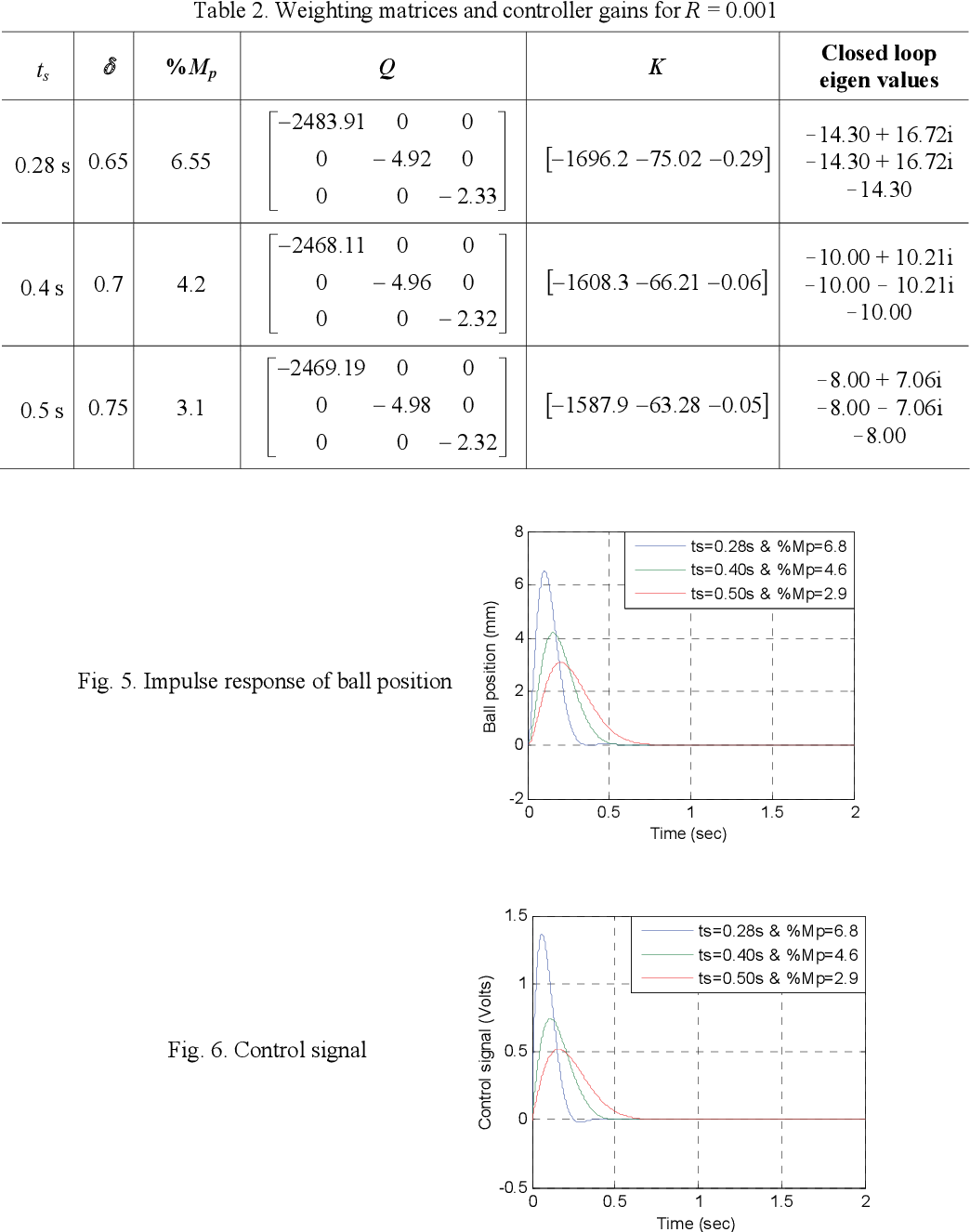
The following image provides a perfect illustration of this trade-off. For a fixed $R$, as the weights in $Q$ are increased, the system responds faster and with less overshoot, but the required control signal becomes much larger.

2. A Systematic Start: Bryson's Rule

So, how do you pick the initial values for $Q$ and $R$? Choosing them randomly is inefficient. A widely used heuristic for a good starting point is Bryson's Rule.

The rule provides a way to scale the penalties based on the maximum acceptable deviations for each state and control input.

As the documentation describes, the rule is as follows:
$Q_{i,i}=\frac{1}{(\text{maximum acceptable value of }{x}_i{)}^2}$
$R_{j,j}=\frac{1}{(\text{maximum acceptable value of }{u}_j{)}^2}$

The diagonal elements of $Q$ and $R$ are set to the inverse of the squared maximum acceptable value for the corresponding state or input. The off-diagonal elements are typically set to zero.

This is a form of normalization. By scaling each component this way, you make a 1-unit deviation in each scaled state or input equally "costly," providing a sensible and balanced starting point for your design.

Example for your Inverted Pendulum:
Let your state vector be $x=[\text{pos},\dot{\text{pos}},\theta ,\dot{\theta }{]}^T$. Suppose your design requirements are:

• Cart position should not deviate more than 0.5 meters.
• Pendulum angle should not deviate more than 0.1 radians ($\approx 5.7^{\circ }$).
• Motor force should not exceed 10 Newtons.

You might not have hard limits for the velocities, so you can estimate them. Let's say max cart velocity is 1 m/s and max pendulum angular velocity is 2 rad/s.

Using Bryson's rule, your initial diagonal $Q$ and $R$ would be:

• $Q_{1,1}(\text{pos})=1/(0.5^2)=4$
• $Q_{2,2}(\dot{\text{pos}})=1/(1^2)=1$
• $Q_{3,3}(\theta )=1/(0.1^2)=100$
• $Q_{4,4}(\dot{\theta })=1/(2^2)=0.25$
• $R_{1,1}(\text{force})=1/(10^2)=0.01$

This gives you a starting point: $Q=\text{diag}([4,1,100,0.25])$ and $R=[0.01]$. Notice that this initial guess already heavily penalizes the pendulum angle $\theta$, which aligns with the physical goal of keeping it upright.

3. The Iterative Design Process

Bryson's rule gives you a good first guess, but LQR design is fundamentally an iterative, trial-and-error process. You start with an initial $Q$ and $R$, simulate the response, and then tune the matrices until the performance meets your requirements.

The following resources show this iterative process in action.

Now, let's look at an example that is directly relevant to your pendulum project. This resource walks through the exact process of tuning $Q$ for an inverted pendulum.

4. Practical Tuning Strategies

Summarizing the process, here is a workflow for tuning your LQR controller:

1. Set an Initial Guess: Use Bryson's Rule to get a reasonable starting point for your diagonal $Q$ and $R$ matrices. If you don't have hard limits, starting with identity matrices ($Q=I,R=I$) is also common.

2. Simulate and Analyze: Run a simulation with your initial controller. Look at the state trajectories and the control input. Does the system meet your performance criteria (settling time, overshoot)? Is the control input within the physical limits of your actuator?

3. Tune the Ratios:

   • Overall Performance: If the response is too slow, increase the overall $Q/R$ ratio. You can do this by multiplying your entire $Q$ matrix by a factor (e.g., 10) or dividing your $R$ matrix by a factor. If the control effort is too high and saturating your actuator, do the opposite (decrease $Q$ or increase $R$).
   • Specific State Performance: If a particular state is not behaving as desired (e.g., too much overshoot, slow to settle), increase the corresponding diagonal element in the $Q$ matrix. This tells the controller to prioritize regulating that specific state.

4. Iterate: Repeat steps 2 and 3. The process is a loop: design -> simulate -> analyze -> repeat. Don't be afraid to make large changes to the weights (factors of 10 or 100) to see a clear effect on the response.

This iterative process, guided by physical intuition about your system, is the essence of practical LQR design.

Conclusion

In this lesson, you've learned the practical art of selecting and tuning the LQR weighting matrices. You now have a framework for translating high-level performance goals into the numbers that define the LQR cost function.

Key Takeaways:

• LQR design is an iterative process of selecting $Q$ and $R$ to balance performance and effort.
• Only the ratio of $Q$ to $R$ matters.
• Bryson's Rule provides a systematic, physics-based method for choosing initial values for $Q$ and $R$.
• Tuning involves adjusting the $Q/R$ ratio for overall aggressiveness and modifying individual diagonal elements of $Q$ to improve the response of specific states.

Preview of the Next Lesson:
We now know how to formulate the LQR problem (Lesson 1) and how to select the design parameters $Q$ and $R$ (this lesson). But we've been treating the lqr command in MATLAB as a black box. In the next lesson, we will peek inside that box to understand how the optimal gain $K$ is actually calculated. We'll introduce the Algebraic Riccati Equation (ARE), the mathematical cornerstone that provides the solution to the LQR problem.