Hello! Welcome to your seventh lesson in the "Advanced Excel for Data Analysis" module.
In our last lesson, you learned how to create charts to visualize data and tell a story. This is a crucial skill for communicating insights. Today, we'll explore another powerful visualization technique that works directly within your data tables, allowing you to spot important information at a glance.
Today's learning outcome: By the end of this lesson, you will be able to apply conditional formatting rules to highlight data trends and outliers.
Instead of creating a separate chart, conditional formatting dynamically changes the appearance of cells (e.g., their color, font style, or by adding icons) based on the data they contain. It's an essential tool for making large tables of data more readable and for quickly drawing attention to key values, such as high-performing sales, projects that are behind schedule, or unusual data points that might be outliers.
1. What is Conditional Formatting?
Before we dive into the "how," let's start with the "what" and "why," which I know you prefer. Conditional formatting is an automated way to make your data speak to you visually.
To get a clear understanding of its purpose and see it in action, let's begin with a short introduction from a video and a quick read.
Conditional Formatting in Excel Tutorial
This brief clip from Kevin Stratvert's tutorial explains what conditional formatting is and why it's so valuable for visualizing trends and patterns directly in your data.
Watch the first 19 seconds of the video (00:00 - 00:19) for a concise overview.
Now, let's solidify that concept with a formal definition and see where to find this feature in Excel.
Conditional Formatting in Excel: A Beginner's Guide
This article from DataCamp, 'Conditional Formatting in Excel: A Beginner's Guide', provides a great written introduction. We'll start with the basics.
Please read the first two sections, 'What is Conditional Formatting?' and 'How It Works: The Basics of Conditional Formatting in Excel'. This will reinforce the concept and show you where the tool is located on the Excel ribbon.
In essence, conditional formatting applies a set of rules to a range of cells. If a cell's value meets the rule's criteria, a specific format is applied automatically.
2. Applying Built-in Formatting Rules
Excel comes with many pre-built rules that are easy to apply and cover most common analytical needs. These rules are excellent for highlighting values, identifying top performers, and adding visual context to your numbers.
The following video provides a practical walkthrough of these features.
Conditional Formatting in Excel Tutorial
Let's return to Kevin Stratvert's tutorial. He demonstrates several of the most useful built-in conditional formatting options.
Watch the following segments to see how to apply different types of rules: Highlight Cells Rules (00:47 - 03:17): See how to highlight cells based on their value (e.g., less than a number) or date. Highlight Duplicates (03:24 - 03:57): Learn how to quickly find duplicate entries, a common task in data cleaning. Top/Bottom Rules (03:57 - 04:39): Discover how to highlight top/bottom values, percentages, or values that are above or below the average. Data Bars, Color Scales, and Icon Sets (04:39 - 05:11): Explore visual styles that turn your cells into mini-charts.
These visual styles—Data Bars, Color Scales, and Icon Sets—are particularly effective for showing relative value and trends at a glance.
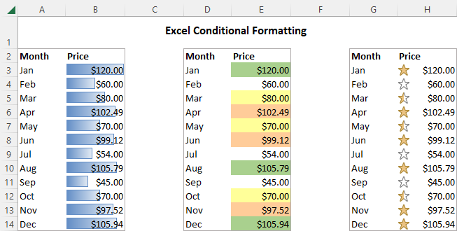
As summarized in the DataCamp article under "Conditional Formatting Styles in Excel", these rules help you:
- Highlight Cells: Pinpoint values greater than, less than, or between certain numbers.
- Top/Bottom Rules: Instantly identify top performers or underachievers.
- Data Bars: Add a bar chart inside each cell to compare magnitudes.
- Color Scales: Create a "heatmap" to show the distribution of values, with colors representing high to low.
- Icon Sets: Use symbols like arrows or traffic lights to indicate performance against a threshold.
3. Using Conditional Formatting to Identify Outliers
One of the most important uses of conditional formatting for a data analyst is identifying outliers. Outliers are data points that are significantly different from other observations and can heavily skew your analysis (for example, by affecting the mean).
You can set up a rule to automatically highlight any values that fall outside a predefined "normal" range.
Finding Outliers In Excel: A Detailed Guide
This article from Acuity Training demonstrates exactly how to use conditional formatting to find outliers.
Read the section 'Methods To Identify Outliers In Excel', focusing specifically on the subsection '1. Conditional Formatting'. This will walk you through setting up rules to highlight values that are 'greater than' an upper limit or 'less than' a lower limit.
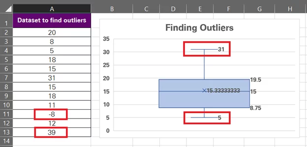
As you can see, conditional formatting makes potential outliers immediately visible for further investigation. We'll cover the statistical methods for calculating these outlier thresholds (like the Interquartile Range or Standard Deviation methods) in a later module on statistics. For now, the key is knowing how to apply the formatting rule once you have those thresholds.
4. Unleashing Power with Formula-Driven Rules
While built-in rules are convenient, you'll often need more complex, custom logic. This is where formula-driven conditional formatting comes in. By writing your own formula, you can create a rule for almost any scenario.
This is a more advanced technique, and understanding the logic behind it is crucial. The following video breaks it down into three simple principles.
Conditional Formatting Formulas - Mystery Solved with 3 Simple Rules
This excellent video from MyOnlineTrainingHub demystifies formula-based conditional formatting by explaining three core rules you need to know.
Watch from the beginning to 03:59. Pay close attention to the explanation of the three rules, especially the third one about absolute and relative references, as this is the most critical concept.
Let's summarize those three essential rules for using formulas:
- The Formula Must Return TRUE or FALSE: Conditional formatting is applied only when your formula evaluates to
TRUE(or a non-zero number). Your formula is essentially asking a yes/no question for each cell. - Select the Range First: Before writing the formula, you must select all the cells you want the formatting to apply to.
- Use Absolute and Relative References Correctly: This is the most important rule. When you write the formula, you write it as if it's only for the top-left cell of your selected range. Excel then automatically adjusts it for all other cells.
- To format an entire row based on a value in a specific column, you must "lock" the column reference with a
$sign. For example, to format row 2 based on the value in cell C2, your formula might be=$C2="Overdue". The$on the column (C) means "always look in column C," while the lack of a$on the row (2) means "check each row individually."
- To format an entire row based on a value in a specific column, you must "lock" the column reference with a
Practice Exercise
Now it's time to put this into practice. Imagine you're managing a list of freelance projects in Excel.
Data:
Create a new Excel sheet and enter the following data:
| Project Name | Client | Status | Due Date | Revenue (EGP) |
|---|---|---|---|---|
| Website Redesign | ABC Corp | Completed | 15-May-24 | 25000 |
| Logo Design | XYZ Inc. | In Progress | 30-Jun-24 | 8000 |
| Market Research | Tech Solutions | Overdue | 01-Jun-24 | 15000 |
| Social Media Ads | Fashion Hub | In Progress | 15-Jul-24 | 12000 |
| Blog Content | ABC Corp | Completed | 25-May-24 | 10000 |
| App Mockup | Tech Solutions | Overdue | 10-Jun-24 | 20000 |
Your Tasks:
- Highlight High-Value Projects: Use a built-in rule to highlight any projects with
Revenue (EGP)greater than 18000 with a green fill. - Visualize Revenue: Apply a Color Scale to the
Revenue (EGP)column to create a heatmap effect, showing the range from low to high revenue. - Flag Overdue Projects: Use a formula-based rule to highlight the entire row in a light red fill for any project where the
Statusis "Overdue". (Hint: Your selection should beA2:E7, and your formula should check the value in column C).
Click here for guidance on the solutions
-
High-Value Projects:
- Select the range
E2:E7. - Go to Home > Conditional Formatting > Highlight Cells Rules > Greater Than...
- Enter
18000and choose "Green Fill with Dark Green Text".
- Select the range
-
Visualize Revenue:
- Select the range
E2:E7. - Go to Home > Conditional Formatting > Color Scales.
- Choose a scale (e.g., the first option, "Green - Yellow - Red Color Scale," though you might reverse it in the settings so green is high).
- Select the range
-
Flag Overdue Projects:
- Select the entire range of data you want to format, which is
A2:E7. - Go to Home > Conditional Formatting > New Rule...
- Select "Use a formula to determine which cells to format".
- In the formula box, enter:
=$C2="Overdue" - Click the "Format..." button, go to the "Fill" tab, and choose a light red color. Click OK.
- The
$before theCis crucial. It tells Excel to always check column C for the status, while the2without a$allows Excel to check each row (row 3, row 4, etc.) in your selection.
- Select the entire range of data you want to format, which is
Conclusion
Excellent work! You've now added another essential data visualization tool to your Excel toolkit. You've learned how to use conditional formatting to make your data tables more intuitive and how to automatically flag trends, patterns, and outliers without needing to build separate charts.
Key Takeaways:
- Conditional formatting automatically applies formatting to cells based on rules you define.
- Built-in rules are great for common tasks like highlighting values, finding duplicates, and applying visual scales (data bars, color scales).
- Formula-based rules offer maximum flexibility, allowing you to create custom logic for complex conditions.
- Correctly using absolute (
$C) and relative (C) references is the key to mastering formula-based formatting, especially for highlighting entire rows.
In our next and final lesson for this module, we will learn how to combine multiple Excel functions in nested formulas to solve complex analytical problems, building directly on the formula logic we explored today.