Hello! Welcome to your sixth lesson in the "Advanced Excel for Data Analysis" module.
In our last lesson, you did an excellent job learning how to use text functions like TRIM, LEFT, RIGHT, and MID to clean and structure messy data. This process, often called data wrangling, is the essential groundwork that makes meaningful analysis possible. Now that you know how to prepare your data, it's time to learn how to tell its story visually.
Today's learning outcome: By the end of this lesson, you will be able to create charts (bar, line, scatter) to visualize data patterns in Excel.
Data visualization is one of the most critical skills for a data analyst. A well-designed chart can reveal trends, patterns, and outliers far more effectively than a table of numbers. It transforms raw data into insights that are easy for anyone to understand, which is key to making data-driven business decisions.
Part 1: Choosing the Right Tool for the Job
Before you create a chart, you need to decide which type of chart best answers your question. Your choice depends on what you want to show: a comparison, a trend over time, or a relationship between variables.
Since you prefer to understand the theory first, let's start with a video that explains the primary purpose of our three key chart types.
How To Choose The Right Graph (Types of Graphs and When To Use Them)
This video from the UNDATABLE channel clearly explains when to use different types of graphs. Pay close attention to the descriptions for bar, line, and scatter plots.
Please watch the following segments: Bar Charts (00:10 - 01:48): Learn why bar and column charts are best for comparing values across different categories. Scatter Plots (03:30 - 04:02): Understand how scatter plots are used to show the relationship or correlation between two numerical variables. Line Charts (04:02 - 04:24): See why line charts are the ideal choice for visualizing trends over time.
To summarize the key ideas:
- Bar/Column Charts: Use these to compare discrete categories. For example, comparing sales figures for different products or regions.
- Line Charts: Use these to show a trend over a continuous interval, most commonly time. For example, tracking monthly website visitors or a stock price over a year.
- Scatter Plots: Use these to investigate the relationship between two different numerical variables. For example, exploring if there is a connection between advertising spend and product sales.
Part 2: Building Charts in Excel
Now that you know when to use each chart, let's learn how to create them in Excel. The process generally follows three steps: select your data, insert the chart, and then customize it for clarity.
The following comprehensive video demonstrates the entire process. It's a bit older (Excel 2010), but the fundamental steps and concepts are almost identical in modern versions of Excel.
Excel 2010 Statistics 07: Charts Basics: Pie, Column, Bar, Line and X-Y Scatter
This video from the 'excelisfun' channel provides a detailed, step-by-step guide to creating charts. We will focus on the sections covering column, bar, line, and scatter charts.
Watch the following sections to see how each chart is built from scratch: Column Charts (08:39 - 12:19): This section shows how to create a vertical column chart to compare categories and how to clean it up. Bar Charts (12:06 - 15:13): Watch how a column chart can be changed to a horizontal bar chart, which can sometimes emphasize differences more strongly. Line Charts (17:21 - 23:46): This part explains how to create a line chart for showing trends and importantly, clarifies the difference between a line chart and a scatter plot. Scatter Plots (23:46 - 29:46): This is a fantastic walkthrough of how to create an XY scatter plot to see the relationship between two number-based variables.
If you prefer a written guide, this article from DataCamp provides clear, modern instructions for creating these charts.
Visualizing Data in Excel | DataCamp
This DataCamp tutorial, 'Visualizing Data in Excel', is a great text-based resource that covers the same ground as the video.
Read the sections titled 'Excel bar charts', 'Excel column charts', 'Excel line charts', and 'Excel scatter plots'. These provide concise, step-by-step instructions for creating each chart type.
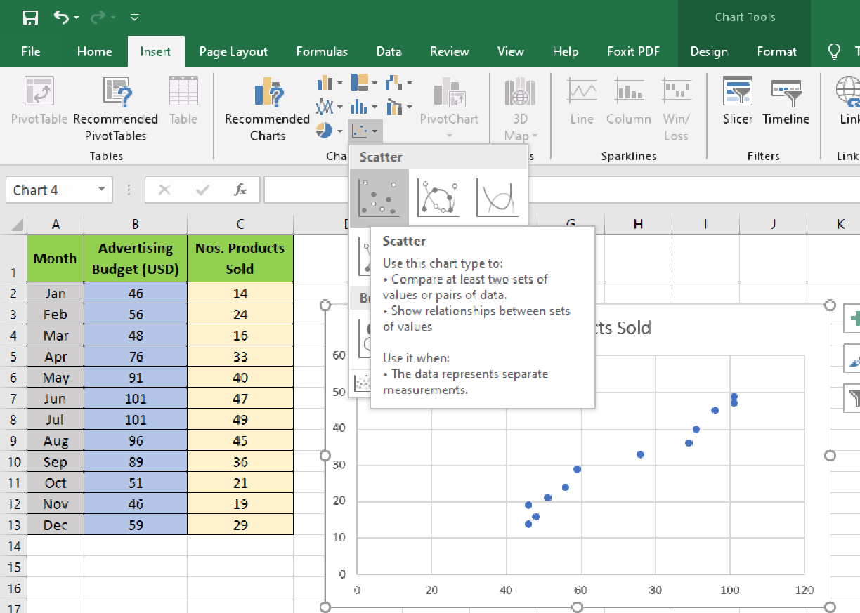
This image shows what the scatter plot creation process looks like in a modern version of Excel.
Part 3: Creating Presentation-Quality Graphs
Creating a chart is easy, but creating an effective chart requires thoughtful refinement. As a data analyst, your goal is to communicate information clearly and concisely. This means removing anything that might distract or mislead your audience—what the famous statistician Edward Tufte calls "chartjunk."
A presentation-quality graph should be:
- Clear: All text should be legible and easy to understand.
- Complete: It must have a title, and axes must be labeled with units.
- Simple: Remove unnecessary elements like distracting gridlines or redundant legends.
This resource provides an excellent guide to transforming a basic chart into a professional one.
Chapter 5 Basic data analysis with Excel
This chapter from the book 'Introduction to Statistics for Economics' has an excellent section on improving the quality of your charts for presentations.
Please read section '5.4.3 Creating presentation-quality graphs'. Focus on the six principles of data visualization and the practical steps shown in the example, such as removing gridlines, modifying the title, and adding labels.
Key customizations to always consider:
- Chart Title: Change the default title to something descriptive that explains what the chart shows.
- Axis Titles: Add titles to your horizontal (X) and vertical (Y) axes to explain what is being measured and in what units (e.g., "Revenue (in EGP)", "Time (Months)").
- Data Labels: Sometimes, adding the exact value to a bar or point can be helpful, but use them sparingly to avoid clutter.
- Legend: Ensure your legend is clear, or remove it if you only have one data series and can describe it in the title.
- Gridlines: Default gridlines are often too prominent. Consider removing them or making them a lighter color to make your data stand out.
Practice Exercise
Let's apply what you've learned. Imagine you are tracking your freelance work with the following dataset.
| Month | Hours Worked | Revenue (EGP) | Clients |
|---|---|---|---|
| Jan | 80 | 12000 | 3 |
| Feb | 95 | 14500 | 4 |
| Mar | 110 | 16000 | 4 |
| Apr | 100 | 15000 | 5 |
| May | 120 | 18500 | 6 |
| Jun | 130 | 20000 | 6 |
Your Task:
Create a new Excel sheet with this data. Then, create three separate charts:
- A column chart to compare the
Revenue (EGP)for eachMonth. - A line chart to show the trend in the number of
Clientsfrom January to June. - A scatter plot to investigate the relationship between
Hours Worked(on the X-axis) andRevenue (EGP)(on the Y-axis).
For each chart, apply the principles of presentation-quality graphs: give it a clear title, label your axes, and remove any unnecessary clutter.
Click here for guidance on the solutions
Here’s a guide to creating the charts:
-
Revenue Column Chart:
- Data: Select the
MonthandRevenue (EGP)columns (A1:A7 and C1:C7). - Chart Type: Insert > Column Chart.
- Customization:
- Title: "Monthly Revenue from Freelance Work (Jan-Jun)"
- Y-Axis Title: "Revenue (EGP)"
- Remove the legend and horizontal gridlines for a cleaner look.
- Data: Select the
-
Client Trend Line Chart:
- Data: Select the
MonthandClientscolumns (A1:A7 and D1:D7). - Chart Type: Insert > Line Chart (choose "Line with Markers").
- Customization:
- Title: "Monthly Growth in Client Numbers"
- Y-Axis Title: "Number of Clients"
- Ensure the X-axis correctly shows the months.
- Data: Select the
-
Hours vs. Revenue Scatter Plot:
- Data: Select the
Hours WorkedandRevenue (EGP)columns (B1:B7 and C1:C7). - Chart Type: Insert > Scatter Chart.
- Customization:
- Title: "Relationship Between Hours Worked and Revenue"
- X-Axis Title: "Hours Worked"
- Y-Axis Title: "Revenue (EGP)"
- Bonus: Right-click on a data point and select "Add Trendline" to see the correlation visually.
- Data: Select the
Conclusion
Fantastic work! You have now learned how to turn clean data into powerful visual stories using Excel's most common chart types. You know not only how to build these charts but, more importantly, why and when to use each one, and how to refine them for maximum clarity and impact. This is a fundamental skill that separates a data manipulator from a true data analyst.
Key Takeaways:
- Bar/Column charts are for comparing values across categories.
- Line charts are for showing trends over time.
- Scatter plots are for exploring relationships between two numerical variables.
- A great chart is simple, clear, and complete, with descriptive titles and labeled axes. Always aim to remove "chartjunk."
In our next lesson, we'll explore another powerful visualization technique in Excel: applying conditional formatting rules to highlight data trends and outliers directly within your data tables. This will give you another tool for quickly spotting important information.