Hello! Welcome back to our journey through advanced Excel.
In our last lesson, we explored the VLOOKUP function. While useful, we also discovered its significant limitations: it can only search in the first column and look to the right, and its reliance on a fixed column number makes it fragile when your data changes. This is a common frustration for analysts.
Today, we'll learn the superior method for performing lookups in Excel: combining the INDEX and MATCH functions. This powerful duo overcomes all of VLOOKUP's main weaknesses, offering a flexible and robust way to find the data you need. By the end of this lesson, you will be able to combine INDEX and MATCH to perform lookups that are impossible with VLOOKUP.
Why INDEX and MATCH are Better
Before we dive into the "how," let's solidify the "why." You already know VLOOKUP can't look to its left. Let's see a practical demonstration of this problem and how INDEX and MATCH solve it.
Data Analyst Explains When to Use VLOOKUP vs XLOOKUP vs INDEX MATCH
This video from data analyst Mo Chen clearly demonstrates the exact moment VLOOKUP fails and introduces INDEX MATCH as the solution. This provides excellent context for why we are learning this new technique.
Watch from 04:36 to 06:50. Notice how the VLOOKUP formula returns an error when trying to find the 'Customer Name' to the left of the 'Customer ID', then see how INDEX MATCH is presented as the answer.
The INDEX and MATCH combination is preferred by data professionals for several key reasons:
- Left or Right Lookup: Unlike
VLOOKUP, you can return a value from a column to the left of your lookup column. This is arguably its biggest advantage. - Stable and Robust: The formula doesn't break if you insert or delete columns in your table. Because you define the lookup and return columns separately, your formulas are much safer and require less maintenance.
- Better Performance: On very large datasets,
INDEX MATCHcan be faster because it only processes the specific lookup and return columns, not the entire table array. - No Size Limit:
VLOOKUPcan fail if your lookup value is longer than 255 characters.INDEX MATCHdoes not have this limitation.
The image below visually contrasts how VLOOKUP breaks and INDEX MATCH holds strong when a new column is inserted.

Deconstructing the Formula: One Function at a Time
Following your preference for understanding the theory first, we'll look at INDEX and MATCH individually before combining them. Think of them as two separate tools that, when used together, become incredibly powerful.
The INDEX Function: Your Data "GPS"
The INDEX function is like a GPS for your spreadsheet. You give it a map (a range of cells) and a set of coordinates (a row number and, optionally, a column number), and it tells you what value exists at that specific location.
Its syntax is: INDEX(array, row_num, [column_num])
array: The "map" where your answer lies.row_num: Which row to go down to.column_num: Which column to go across to (this is optional if your array is just one column).
To see this explained with a great analogy, please watch the first part of this next video.
How to use Excel Index Match (the right way)
This video from Leila Gharani provides a clear, step-by-step breakdown of each function. We'll start with her explanation of INDEX.
Watch from 00:52 to 04:22. Pay attention to the 'GPS and map' analogy. Notice how INDEX simply retrieves a value based on the row and column numbers you give it.
As you can see, INDEX is great at fetching data, but it has a problem: it needs to be told the exact row and column numbers. How can we find those numbers automatically? That's where MATCH comes in.
The MATCH Function: Your "Position Finder"
The MATCH function does one simple job: it looks for a value in a single row or column and tells you its relative position (i.e., the row or column number).
Its syntax is: MATCH(lookup_value, lookup_array, [match_type])
lookup_value: The value you're looking for.lookup_array: The single column or row where you're looking.match_type:0for an exact match (most common),1for less than,-1for greater than. Just like withVLOOKUP, we will almost always use0for an exact match.
Let's return to the video to see how MATCH works.
How to use Excel Index Match (the right way)
Now, let's see how the MATCH function finds the position number that INDEX needs.
Watch from 04:22 to 06:27. The key takeaway here is that MATCH returns a number, which is precisely the input that the 'row_num' argument of the INDEX function requires.
Combining INDEX and MATCH: The Complete Formula
Now we put the pieces together. We use MATCH to find the correct row number, and we feed that number directly into the INDEX function to retrieve our value.
The structure looks like this:
=INDEX(column_to_return_a_value_from, MATCH(what_you_want_to_look_up, column_to_look_up_against, 0))
- The
MATCHpart finds the row number of your lookup item. - The
INDEXpart takes that row number and returns the value from the corresponding row in the return column.
Watch the next section of the video to see this combination built step-by-step.
How to use Excel Index Match (the right way)
This is the core of the lesson. You'll see how to 'nest' the MATCH function inside the INDEX function to create a dynamic lookup.
Watch from 06:27 to 08:07. Notice how the ranges for INDEX and MATCH must have the same height (number of rows) to be in sync.
To solidify this, let's look at a clear textual explanation.
Excel INDEX MATCH vs. VLOOKUP - formula examples
The article 'Excel INDEX MATCH vs. VLOOKUP' from Ablebits.com provides a fantastic written breakdown of the formula. Reading this will reinforce what you just saw in the video.
Read the sections 'Excel INDEX and MATCH functions - the basics' and 'How to use INDEX MATCH function in Excel'. Focus on how the output of MATCH becomes the input for INDEX.
Advanced Use: Two-Way Lookup
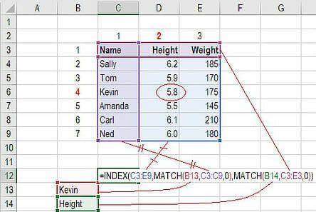
The flexibility of INDEX MATCH doesn't stop there. What if you need to look up a value based on both a row and a column criterion? For example, finding the sales figure for a specific product in a specific month. You can do this by using MATCH twice within one INDEX function: one MATCH for the row and one for the column.
The structure is:=INDEX(full_table_array, MATCH(row_lookup_value, row_lookup_column, 0), MATCH(column_lookup_value, column_lookup_row, 0))
This is a powerful technique for matrix-style lookups.
How to use Excel Index Match (the right way)
Let's see the final demonstration from Leila Gharani's video, where she builds a flexible two-way lookup.
Watch from 08:07 to 10:31. See how a second MATCH function is added to the formula to dynamically find the correct column number.
The image below gives another clear, static view of how this two-way lookup works.
Practice Exercise
Let's use the same tables from our last lesson to solve the problem that VLOOKUP couldn't handle.
Table 1: Orders
| Order ID | Customer ID | Customer Name |
|---|---|---|
| 101 | C03 | Omar Adel |
| 102 | C01 | Ali Hassan |
| 103 | C04 | Salma Ibrahim |
| 104 | C02 | Fatima Said |
Table 2: Customers
| Region | Customer Name | Customer ID |
|---|---|---|
| Cairo | Ali Hassan | C01 |
| Alexandria | Fatima Said | C02 |
| Giza | Omar Adel | C03 |
| Cairo | Salma Ibrahim | C04 |
Notice I've rearranged Table 2 so Customer ID is no longer the first column.
Your task:
In a new sheet, you want to find the Customer ID for "Fatima Said".
- Your lookup value is "Fatima Said".
- Write an
INDEX MATCHformula to find herCustomer IDfrom Table 2.
Hint:
- The
INDEXarraywill be theCustomer IDcolumn. - The
MATCHfunction will look for "Fatima Said" in theCustomer Namecolumn.
This is a right-to-left lookup that VLOOKUP would fail.
Conclusion
You have now learned one of the most powerful and essential formula combinations in Excel for data analysis.
Key Takeaways:
INDEX MATCHis a combination whereMATCHfinds the position of an item, andINDEXretrieves the value at that position.- It overcomes
VLOOKUP's biggest flaws: it can look left, and it is not affected by the insertion or deletion of columns. - The basic structure is
=INDEX(return_column, MATCH(lookup_value, lookup_column, 0)). - You can extend this with a second
MATCHfor powerful two-way lookups.
As a data analyst, you will encounter lookup tasks constantly. By mastering INDEX and MATCH, you have a reliable and flexible tool to handle almost any scenario.
In our next lesson, we will shift from lookup formulas to a powerful built-in tool for summarizing and aggregating data: Pivot Tables. This will allow us to quickly group and analyze large datasets without writing complex formulas.