Hello! Welcome to the first lesson in our "Advanced Excel for Data Analysis" module.
In your previous work with data entry and document formatting, you've likely had to manually cross-reference information between different lists or sheets. This is a common but time-consuming task. Today, we'll learn a powerful function that automates this process, saving you significant time and reducing errors.
This lesson covers VLOOKUP, one of the most well-known functions in Excel. We'll explore how to use it to retrieve data from a table and, just as importantly, we will discuss its significant limitations. Mastering VLOOKUP is a fundamental step in moving from basic data handling to performing genuine data analysis in Excel.
What is VLOOKUP?
VLOOKUP stands for Vertical Lookup. Its purpose is to search for a specific piece of information (the lookup_value) in the first column of a data table. Once it finds a match, it moves horizontally to the right along that same row and returns a value from a column you specify.
Think of it like looking up a person's name in a directory: you find the name in the first column, then scan across that row to find their phone number or address.
The VLOOKUP function has four components, called arguments, that you need to provide:
=VLOOKUP(lookup_value, table_array, col_index_num, [range_lookup])
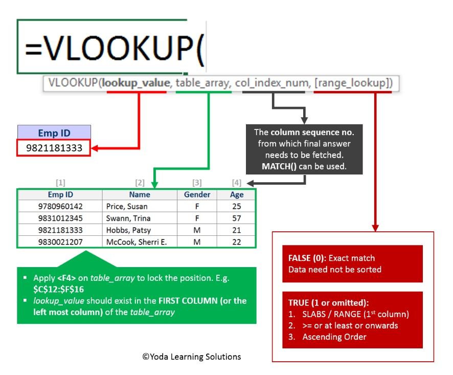
lookup_value: The value you want to search for. This is your starting point.table_array: The range of cells that contains your data. Crucially, the column containing yourlookup_valuemust be the first column in this range.col_index_num: The column number within yourtable_arrayfrom which you want to retrieve a value. The first column is 1, the second is 2, and so on.[range_lookup]: This is an optional but critical argument. It tells Excel whether you want an exact match (FALSE) or an approximate match (TRUE). For most data analysis tasks, you will want an exact match.
The image below provides an excellent visual summary of how these arguments fit together.
Performing an Exact Match with VLOOKUP
Now that you have the theory, let's see VLOOKUP in action. The most common use case is finding an exact match, such as looking up a specific customer ID to find their name or pulling a product price using its unique product code.
Please watch the following video to see how to build a VLOOKUP formula from scratch.
How to Use VLOOKUP in Excel (free file included)
In this video, 'How to Use VLOOKUP in Excel' by Leila Gharani, you will see a step-by-step demonstration of the function. Pay close attention to how each of the four arguments is selected and why.
Watch the segment from the beginning until 07:01. The first part (until 05:28) covers the basic formula and the importance of using 'FALSE' for an exact match. It also shows you a critical technique: how to 'lock' your table array reference using the F4 key to prevent errors when copying the formula. The second part (until 07:01) demonstrates how this works when your data is on another sheet.
As you saw, getting the range_lookup argument right is essential. If you leave it blank or set it to TRUE, Excel defaults to an "approximate match," which can give you incorrect results if you're expecting an exact match. A good habit is to always specify FALSE (or its equivalent, 0) unless you have a specific need for an approximate match.
The Limitations of VLOOKUP
While VLOOKUP is incredibly useful, it's not perfect. Understanding its limitations is just as important as knowing how to use it, as this will help you avoid common pitfalls and know when to use a more powerful tool (which we'll cover in the next lesson).
Please read the following sections from the article "23 things you should know about VLOOKUP" to understand its main drawbacks.
23 things you should know about VLOOKUP
This article from Exceljet provides a clear, in-depth look at the nuances of VLOOKUP. We will focus on its key limitations.
Please read sections 2, 3, 4, and 6. They are titled: '2. VLOOKUP only looks right' '3. VLOOKUP finds the first match' '4. VLOOKUP is not case-sensitive' '6. Caution: VLOOKUP uses approximate match by default' Focus on understanding why each of these points is a limitation in data analysis.
To summarize and add a few more practical points, here are the main limitations of VLOOKUP:
- It Can Only Look to the Right: The lookup column must be the leftmost column in your table array. You cannot use
VLOOKUPto find a value in a column and return data from a column to its left. - It Returns the First Match Only: If your lookup column contains duplicates,
VLOOKUPwill stop at the first match it finds and ignore all others. - Column Index Number is "Hard-Coded": If you specify column
3for your result and later insert a new column into your table,VLOOKUPwill not automatically update. It will still be looking at the 3rd column, which might now contain the wrong data, breaking your analysis silently. - Dangerous Default: As mentioned, it defaults to an approximate match (
TRUE), which requires your data to be sorted and can lead to incorrect results if you're not careful. - Performance: On very large datasets (hundreds of thousands of rows), multiple
VLOOKUPformulas can slow down your workbook.

Troubleshooting and Other Use Cases
Knowing the limitations helps in troubleshooting. Common errors like #N/A (value not found) can happen because the value genuinely doesn't exist, or due to formatting issues like extra spaces or numbers stored as text.
The same video from earlier has an excellent section on identifying and solving these common errors. It also provides an example of when to use an approximate match.
How to Use VLOOKUP in Excel (free file included)
Let's return to Leila Gharani's video to learn about troubleshooting and the proper use of approximate matches.
Watch the segments from 07:01 to 14:24. The first part (07:01 - 09:12) explains how to use 'TRUE' for an approximate match, like assigning grades based on scores. The second part (09:12 - 14:24) covers common errors and how to fix them, including a useful tip on using the TRIM function inside your formula.
Practice Exercise
Let's apply what you've learned. Imagine you have two sets of data.
Table 1: Orders
| Order ID | Customer ID |
|---|---|
| 101 | C03 |
| 102 | C01 |
| 103 | C04 |
| 104 | C02 |
Table 2: Customers
| Customer ID | Customer Name | Region |
|---|---|---|
| C01 | Ali Hassan | Cairo |
| C02 | Fatima Said | Alexandria |
| C03 | Omar Adel | Giza |
| C04 | Salma Ibrahim | Cairo |
Your task:
- In the "Orders" table, create a new column called "Customer Name".
- In this new column, write a
VLOOKUPformula to pull the correctCustomer Namefrom the "Customers" table by matching theCustomer ID.
Challenge Question: Could you use VLOOKUP to find which Customer ID corresponds to the name "Fatima Said"? Why or why not?
Think about the "left-to-right" limitation we discussed. The answer is that you cannot use a standard VLOOKUP, because the Customer Name column is not the first column in the Customers table.
Conclusion
In this lesson, you've learned one of the most fundamental functions for data lookup in Excel.
Key Takeaways:
VLOOKUPis used to search for a value in the first column of a table and return a corresponding value from a column to the right.- The formula requires four arguments:
lookup_value,table_array,col_index_num, andrange_lookup. - For accurate, predictable results when looking up unique IDs, always set the
range_lookupargument toFALSEor0for an exact match. - Be mindful of
VLOOKUP's major limitations: it only looks right, it's fragile if columns are inserted, and it only finds the first match.
These limitations are significant, but don't worry. In our next lesson, we will learn a more powerful and flexible method using two functions together: INDEX and MATCH. This combination overcomes all of VLOOKUP's main weaknesses and is the preferred method for many data analysts.