Understanding Space Complexity

What is Space Complexity?

Just as time complexity describes the growth rate of an algorithm's runtime, space complexity describes the growth rate of the memory it requires. We use the same Big-O notation to express this relationship.

However, there's an important distinction to make: total space versus auxiliary space.

• Input Space: The memory used to store the input data itself. For a function that takes a vector of size n, the input space is $O(n)$.
• Auxiliary Space: The extra or temporary memory that an algorithm uses during its execution. This includes variables, data structures, and the memory used by function calls.
• Total Space Complexity: The sum of the input space and the auxiliary space.

In coding interviews, when an interviewer asks for the "space complexity," they are most often interested in the auxiliary space. This is the memory you are adding to solve the problem. Let's clarify this with a short video.

The key takeaway is that we analyze the memory our algorithm allocates in addition to the inputs it is given.

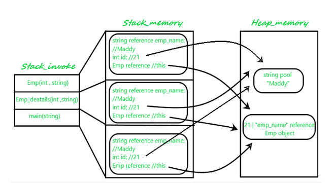
To understand where this space is allocated in a C++ program, it helps to have a basic mental model of the two main memory regions: the stack and the heap.

• The Stack: This is where local variables and function call information are stored. Memory is allocated and deallocated automatically as functions are called and return. It's fast but limited in size.
• The Heap: This is a large pool of memory used for dynamic allocation (e.g., when you use new in C++ or when containers like std::vector need to grow). You or the container's logic are responsible for managing this memory.

Analyzing Iterative Algorithms

Let's start by analyzing the space complexity of some iterative algorithms, which primarily use memory for variables and data structures.

O(1) — Constant Space

An algorithm has constant space complexity if its memory usage does not depend on the input size n. It uses a fixed amount of memory for its variables.

Consider this function that sums the elements of an array:

int sumArray(int arr[], int n) {
    int sum = 0; // O(1) space for 'sum'
    int i = 0;   // O(1) space for 'i'

    for (i = 0; i < n; i++) {
        sum += arr[i];
    }
    return sum;
}

The input arr takes $O(n)$ space, but the auxiliary space is constant. We only declare two integer variables, sum and i. Whether the array has 10 elements or 10 million, the memory needed for these two variables remains the same. Therefore, the auxiliary space complexity is $O(1)$. An algorithm with $O(1)$ auxiliary space is often called an in-place algorithm.

For more examples of common algorithms with $O(1)$ space complexity, you can review the following resource.

O(n) — Linear Space

Linear space complexity occurs when the amount of auxiliary memory an algorithm needs grows proportionally with the input size n. This often happens when you create a new data structure (like a vector or a map) that stores n elements.

A classic example is counting the frequency of elements in an array. A common approach is to use a hash map (std::unordered_map in C++) to store each unique element and its count.

Space Complexity of Recursive Algorithms

When analyzing recursive algorithms, the primary source of auxiliary space is the function call stack. Each time a function calls itself, a new "stack frame" is pushed onto the stack. This frame stores the function's local variables, parameters, and the return address. The space complexity is determined by the maximum number of stack frames present at any one time, which corresponds to the maximum depth of the recursion.

A fantastic video from CodeHelp breaks down the space analysis for several key recursive algorithms.

An Important Interview Tip: Don't Modify Your Inputs

It can be tempting to save space by modifying the input array or data structure directly, thus achieving $O(1)$ auxiliary space. However, unless the interviewer explicitly allows it, this is generally considered bad practice. In real-world software engineering, the function you write might be part of a larger system where other components depend on the input data remaining unchanged.

This is a sign of good software engineering hygiene that interviewers appreciate. Watch this final clip for a clear explanation of this principle.

Conclusion

You now have a complete framework for analyzing the complexity of algorithms in terms of both time and space. This dual understanding is fundamental to designing efficient solutions and is a core expectation in technical interviews.

Key Takeaways:

• Space Complexity measures how an algorithm's memory usage scales with input size, expressed using Big-O notation.
• It's critical to distinguish between total space (including inputs) and auxiliary space (extra memory used). Interviewers usually care about auxiliary space.
• Iterative algorithms use space for variables and data structures. Common complexities are $O(1)$ (constant) and $O(n)$ (linear).
• Recursive algorithms use space on the call stack. The space complexity is determined by the maximum recursion depth. This leads to $O(n)$ for linear recursion (like factorial) and $O(\log n)$ for divide-and-conquer algorithms like binary search.
• In an interview, avoid modifying input data unless explicitly told to. It demonstrates good software engineering practice.

In the next lesson, we will add another layer of nuance to our analysis by learning to compare algorithms based on their best-case, worst-case, and average-case complexity, which applies to both time and space.