Big-O Analysis of Iterative Algorithms

What is Time Complexity and Why Does It Matter?

Imagine you've written a search function for an e-commerce site. It works perfectly with 100 products. But when the inventory grows to 100,000 products, the search slows to a crawl, and users start to complain. The code is correct, but it doesn't scale. This is the core problem that time complexity analysis helps us solve before we run into trouble.

Big-O notation is the language we use to talk about this. It doesn't measure the exact time in seconds an algorithm takes to run—that depends on the hardware, the programming language, and many other factors. Instead, it describes the growth rate of the runtime as the input size, which we'll call n, gets larger. It specifically describes the upper bound or the worst-case scenario.

To get a feel for what this means, I recommend starting with this short segment from a video by NeetCode, a popular resource for interview preparation.

The key takeaway is that we're interested in the "order of" growth. An algorithm with a complexity of $O(2n)$ and one with $O(n)$ are both considered to have $O(n)$ complexity because they both grow linearly. As n becomes very large, the dominant term in the complexity function is the only one that matters.

This graph visually demonstrates why this is so important.

As you can see, an algorithm with $O(n^2)$ complexity becomes drastically slower than an $O(n)$ or $O(\log n)$ algorithm as the input size n grows. In a coding interview, choosing an algorithm from the "better" side of this chart is often the main challenge.

Analyzing Basic Iterative Structures

Let's start analyzing some real C++ code. Since you're comfortable with loops, we'll begin there. Most time complexity analysis for iterative algorithms boils down to counting how many times the statements inside a loop are executed as a function of the input size n.

O(1) — Constant Time

An algorithm has constant time complexity if its execution time does not change regardless of the input size. These are the most efficient operations.

// Returns the first element of a vector.
// The size of the vector does not affect how long this takes.
int getFirstElement(const std::vector<int>& data) {
    if (data.empty()) {
        throw std::runtime_error("Vector is empty");
    }
    return data[0]; // This is an O(1) operation
}

Accessing an element in a std::vector by its index is an $O(1)$ operation. The computer can calculate the memory address of data[0] (or any data[i]) directly, so it doesn't matter if the vector has 10 elements or 10 million.

O(n) — Linear Time

This is one of the most common complexities. The runtime grows in direct proportion to the input size n. If the input doubles, the runtime roughly doubles. This typically occurs when we need to iterate through all elements of a collection once.

// Finds the maximum value in a vector.
int findMaximum(const std::vector<int>& data) {
    if (data.empty()) {
        throw std::runtime_error("Vector is empty");
    }
    int maximum = data[0]; // O(1)
    // The loop runs 'n' times, where n is data.size()
    for (int value : data) { // O(n)
        if (value > maximum) { // O(1) inside the loop
            maximum = value;
        }
    }
    return maximum;
}

In this example, the for loop runs data.size() times. If we call data.size() as n, the total time is roughly proportional to n. The work inside the loop is constant time, $O(1)$. Therefore, the total complexity is $n\times O(1)$, which is $O(n)$.

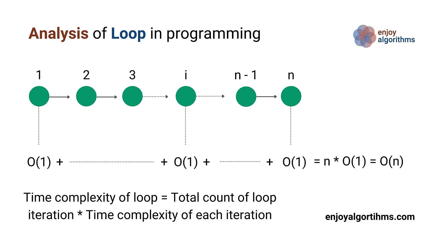
A common point of confusion is what happens if the loop doesn't increment by one. The following video by Abdul Bari clarifies this point well.

What if you have two separate, non-nested loops?

void processTwoVectors(const std::vector<int>& vec1, const std::vector<int>& vec2) {
    int n = vec1.size();
    int m = vec2.size();

    // First loop runs n times
    for (int i = 0; i < n; ++i) {
        // O(1) work
    }

    // Second loop runs m times
    for (int i = 0; i < m; ++i) {
        // O(1) work
    }
}

In this case, the loops are sequential, not nested. We add their complexities. The total time complexity is $O(n+m)$. We don't simplify this to $O(n)$ unless we know that m is always proportional to n, because n and m could be independent and vary wildly.

Analyzing Nested Loops

Things get more interesting when we nest loops. This is where complexities like $O(n^2)$ often appear.

O(n²) — Quadratic Time

A common pattern for quadratic complexity is a loop nested inside another loop, where both iterate up to n.

// Checks if a vector contains duplicate values.
bool hasDuplicate(const std::vector<int>& data) {
    int n = data.size();
    for (int i = 0; i < n; ++i) {       // Outer loop runs n times
        for (int j = i + 1; j < n; ++j) { // Inner loop runs... how many times?
            if (data[i] == data[j]) {
                return true;
            }
        }
    }
    return false;
}

Notice the inner loop starts from j = i + 1. This means the number of its iterations depends on the outer loop's variable, i.

• When i = 0, the inner loop runs n-1 times.
• When i = 1, the inner loop runs n-2 times.
• ...
• When i = n-2, the inner loop runs 1 time.

The total number of operations is the sum $(n-1)+(n-2)+...+1$. This is a well-known arithmetic series that sums to $\frac{(n-1)n}{2}$, which expands to $\frac{1}{2}{n}^2-\frac{1}{2}n$.

Following the rules of Big-O, we drop the constant factor ($\frac{1}{2}$) and the non-dominant term ($-\frac{1}{2}n$), leaving us with $O(n^2)$.

To really solidify this concept, let's look at two different but complementary explanations.

1. The Formal Derivation: Abdul Bari provides a clear, step-by-step trace and derivation.

2. The Intuitive Visualization: NeetCode offers a more visual, intuitive way to think about this sum.

A Look at Other Common Iterative Complexities

Not all loops are linear or quadratic. Let's explore two other important patterns that can arise in iterative algorithms.

O(log n) — Logarithmic Time

Logarithmic complexity is a hallmark of highly efficient algorithms. It typically appears when the algorithm halves the size of the input it has to consider in each iteration. The classic example is binary search on a sorted array.

The number of times you can divide n by 2 until you get to 1 is given by ${\log }_{2}n$. In Big-O notation, the base of the logarithm is considered a constant factor, so we simply write $O(\log n)$.

O(√n) — Square Root Time

Sometimes, the loop control variable changes in a non-linear way, leading to less obvious complexities. Consider this code:

int i = 0;
int p = 0;
while (p <= n) {
    i++;
    p = p + i;
}

Here, the while loop continues as long as p is less than or equal to n. But p doesn't grow linearly; it grows by i, which itself is incrementing.

• After 1 iteration: p = 1
• After 2 iterations: p = 1 + 2 = 3
• After 3 iterations: p = 1 + 2 + 3 = 6
• After k iterations: p = 1 + 2 + ... + k = k(k+1)/2

The loop stops when p > n. So, we're looking for the value of k where $k(k+1)/2\approx n$. This simplifies to $k^2\approx 2n$, or $k\approx \sqrt{2n}$. Dropping the constant, the number of iterations k is proportional to $\sqrt{n}$, making the time complexity $O(\sqrt{n})$.

A Practical Summary for Interviews

When you're in an interview, you need a quick way to analyze code. Here's a practical guide based on what we've covered.

In a typical 45-minute coding interview, you'll be given a problem with input constraints. For example, n might be up to 10^5. A modern computer can perform roughly 10^8 operations per second.

• An $O(n^2)$ solution would require $(10^5{)}^2=10^{10}$ operations, which is far too slow.
• An $O(n\log n)$ solution would require roughly $10^5\times {\log }_2(10^5)\approx 10^5\times 17$, which is about $1.7\times 10^6$ operations. This is perfectly acceptable.
• An $O(n)$ solution would be even better.

This practical estimation is crucial for guiding you toward an optimal solution.

Conclusion

In this lesson, we established the importance of time complexity and Big-O notation as tools for evaluating algorithms, a critical skill for coding interviews. You've learned how to analyze iterative C++ code and determine its time complexity by examining its loop structures.

Key Takeaways:

• Big-O notation describes the growth rate of an algorithm's runtime in the worst case as the input size n increases.
• We simplify complexity by dropping constants and non-dominant terms.
• A single loop iterating through n elements is typically $O(n)$.
• Sequential loops have their complexities added ($O(n+m)$).
• Nested loops have their complexities multiplied (often leading to $O(n^2)$).
• Algorithms that reduce the problem size by a constant factor (e.g., halving it) in each step are often $O(\log n)$.
• Complex loop structures can lead to other complexities like $O(\sqrt{n})$.

We've focused exclusively on time complexity—how long an algorithm takes. However, performance isn't just about speed; it's also about memory. In the next lesson, we will explore space complexity, which measures how an algorithm's memory usage scales with its input size.