Analyzing Algorithm Complexities

The Three Scenarios of Performance

An algorithm doesn't have a single, universal runtime. Its efficiency is a function of its input. To capture this variability, we analyze three distinct scenarios.

• Best Case: The input that allows an algorithm to finish in the minimum number of steps. This is the algorithm's most optimal performance.
• Worst Case: The input that forces an algorithm to execute the maximum number of steps. This is the performance guarantee—the algorithm will never be slower than this.
• Average Case: The expected performance over all possible inputs. This gives a realistic estimate of an algorithm's behavior in practice.

Let's ground these definitions in a concrete example you're familiar with: linear search.

// A simple linear search function in C++
int linearSearch(int arr[], int n, int target) {
    for (int i = 0; i < n; i++) {
        if (arr[i] == target) {
            return i; // Element found
        }
    }
    return -1; // Element not found
}

What are the best, worst, and average cases for this function?

• Best Case: The target is the very first element, arr[0]. The loop runs only once.
• Worst Case: The target is the last element, arr[n-1], or it's not in the array at all. The loop must run n times.
• Average Case: The target is somewhere in the middle of the array. On average, we'd expect to check about n/2 elements.

To formalize these ideas, please read the following brief article. It defines the three cases and provides C++ examples for several algorithms.

The renowned instructor Abdul Bari provides an excellent, detailed walkthrough of analyzing linear search. His explanation of how to calculate the average case complexity is particularly insightful.

Notations for Bounds: O, Ω, and Θ

Now we need to connect these cases to the asymptotic notations we've been using. There is a very common and critical point of confusion here that we must clarify. Many people mistakenly believe:

• Big-O is for the worst case.
• Big-Omega ($\Omega$) is for the best case.
• Big-Theta ($\Theta$) is for the average case.

This is incorrect.

Big-O, Big-Omega, and Big-Theta are tools for describing the bounds of a function's growth rate, not the performance cases themselves.

• Big-O ($O$) Notation (Upper Bound): This describes a growth rate that is at most as fast as a certain function. It sets a ceiling. An algorithm with a worst-case of $n$ comparisons is $O(n)$, but it's also technically $O(n^2)$ because $n^2$ grows faster. We always prefer the tightest possible upper bound, which is $O(n)$.
• Big-Omega ($\Omega$) Notation (Lower Bound): This describes a growth rate that is at least as fast as a certain function. It sets a floor.
• Big-Theta ($\Theta$) Notation (Tight Bound): This describes a growth rate that is exactly the same as a certain function. An algorithm is $\Theta (f(n))$ if it is both $O(f(n))$ and $\Omega (f(n))$. It is "sandwiched" between upper and lower bounds of the same order.

The following video offers a clear, mathematical breakdown of these three notations.

So, how do we correctly apply these notations to our analysis cases? You can use any notation to describe any case.

Let's revisit linear search:

• Best Case: The runtime is constant (e.g., 1 comparison). We can say the best-case complexity is $\Theta (1)$, which implies it is also $O(1)$ and $\Omega (1)$.
• Worst Case: The runtime is linear (e.g., n comparisons). We can say the worst-case complexity is $\Theta (n)$, which implies it is also $O(n)$ and $\Omega (n)$.

To solidify this crucial point, let's return to Abdul Bari's video, where he explicitly debunks this common misconception.

Why Worst-Case Analysis Dominates

While it's important to understand all three cases, in the world of software engineering and coding interviews, worst-case complexity is paramount. Why? Because it provides a performance guarantee. When you say an algorithm is $O(n^2)$, you are assuring your team that no matter what input is thrown at it, its runtime will not grow faster than a quadratic curve. This allows you to build predictable and reliable systems.

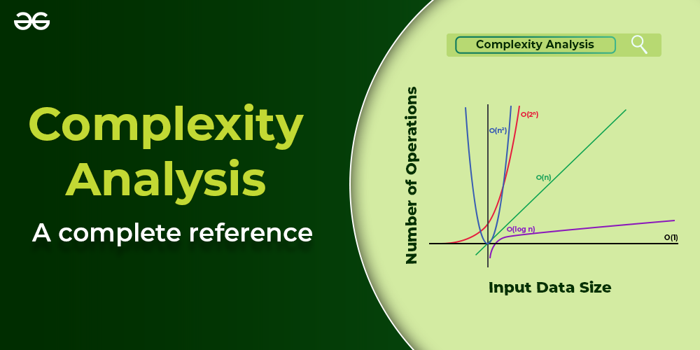
This practical focus is explained well in the following short reading.

To see how this plays out across different algorithms, consider the following table. It's a common sight in computer science resources and summarizes the complexities for several fundamental algorithms you will soon be implementing.

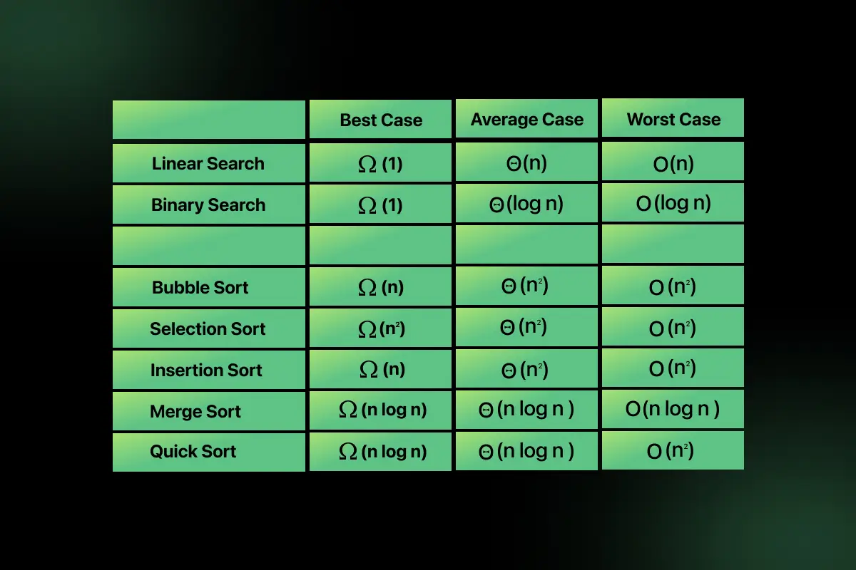
In this table, you'll see a common convention where $\Omega$ is used for the best case, $\Theta$ for the average case, and $O$ for the worst case. While convenient shorthand, you now know the deeper truth: these notations are about bounds, and the use of $O$ for the worst case reflects the industry's focus on guaranteeing an upper bound on performance.

Conclusion

In this lesson, you've added a critical dimension to your understanding of algorithmic analysis. You've moved beyond a single complexity measure to a more nuanced view that accounts for an algorithm's behavior under different conditions.

Key Takeaways:

• An algorithm's performance is analyzed in three main scenarios: best-case, average-case, and worst-case.
• Big-O ($O$), Big-Omega ($\Omega$), and Big-Theta ($\Theta$) are notations for mathematical bounds (upper, lower, and tight), and can be applied to any of the three cases. They are not synonymous with worst, best, and average cases.
• In practice, worst-case analysis is the most important because it provides a reliable performance guarantee, which is essential for building robust software.
• Different algorithms can have vastly different profiles. Some, like Merge Sort, are consistent across all cases, while others, like Quicksort, have a much better average-case performance than their worst-case.

In our next lesson, we will explore another fundamental concept in algorithm design: the time-space trade-off. You'll see how we often can achieve a faster runtime ($O(n)$ instead of $O(n^2)$, for example) by using more memory, a crucial decision-making process in solving complex problems.