Time-Space Trade-offs in Data Structures

The Core Concept: Trading Speed for Memory

In an ideal world, every algorithm would be both lightning-fast and incredibly memory-efficient. In reality, we often have to choose one priority over the other. This decision is the essence of the time-space trade-off.

• A time-efficient algorithm minimizes the number of operations, often by pre-calculating and storing results in memory to avoid re-computation. This uses more space.
• A space-efficient algorithm minimizes memory usage, often by re-calculating values on the fly as needed. This takes more time.

To get a formal introduction to this idea, please read the following article from GeeksforGeeks. It defines the concept and gives several examples.

The idea of using a "lookup table" to store pre-computed answers is the most common and powerful application of the time-space trade-off you'll encounter. Let's see this in action with a problem that is a staple of coding interviews.

Case Study: The "Two Sum" Problem

The "Two Sum" problem is a perfect illustration of the time-space trade-off. Here is the problem statement:

Given an array of integers nums and an integer target, return the indices of the two numbers such that they add up to target. You may assume that each input would have exactly one solution, and you may not use the same element twice.

Let's consider an example: nums = [2, 7, 11, 15] and target = 9. The answer is [0, 1] because nums[0] + nums[1] == 9.

Approach 1: The Brute-Force Solution (Low Space, High Time)

The most straightforward solution is to check every possible pair of numbers.

1. Take the first number.
2. Iterate through all the other numbers and check if their sum equals the target.
3. If no pair is found, take the second number and repeat the process.

This involves nested loops. For an array of size $n$, the outer loop runs $n$ times, and the inner loop runs roughly $n$ times for each of those.

• Time Complexity: $O(n^2)$. This is slow for large arrays.
• Space Complexity: $O(1)$. We are not using any significant extra memory besides a few variables.

Approach 2: The Hash Table Solution (High Space, Low Time)

Can we do better than $O(n^2)$? What if we could check if a number's complement (target - current_number) exists in the array in constant time? This is exactly what a hash table allows us to do.

The algorithm becomes:

1. Create an empty hash table (in C++, an unordered_map) to store numbers we've seen and their indices.
2. Iterate through the array one element at a time.
3. For each number x, calculate its required complement: y = target - x.
4. Check if y exists in the hash table.
   • If it does, we've found our pair! We can return the index of y (which we stored in the hash table) and the index of the current number x.
   • If it doesn't, add the current number x and its index to the hash table so we can find it in future iterations.

Let's trace this with nums = [2, 7, 11, 15] and target = 9.

1. i=0, num=2. Complement is 9 - 2 = 7. Is 7 in the map? No. Add {2: 0} to the map.
2. i=1, num=7. Complement is 9 - 7 = 2. Is 2 in the map? Yes! It's at index 0. We found the pair. Return [0, 1].

The single pass through the array gives us a much better time complexity.

• Time Complexity: $O(n)$. Each lookup and insertion in a hash table takes, on average, $O(1)$ time. We do this for each of the $n$ elements.
• Space Complexity: $O(n)$. In the worst case, we might store all $n$ elements in the hash table.

We've traded $O(n)$ space to reduce our time from $O(n^2)$ to $O(n)$—a classic and highly effective time-space trade-off.

The instructor in the following video from the "take U forward" channel gives an excellent walk-through of these two approaches.

To see how you would frame this discussion in an interview, read the following section from the AlgoCademy blog.

The Engine Behind the Speed: Hash Tables

We've established that hash tables are fast, but why? It comes down to their internal structure. A hash table is fundamentally an array, but instead of using an index like 0, 1, 2, it uses a special hash function to convert a key (like a string "Berlin" or a number 7) into an array index.

When you want to store or find a value, the hash table:

1. Takes your key.
2. Passes it through the hash function to get an index.
3. Goes directly to that index in the underlying array.

This direct access is an $O(1)$ operation. However, sometimes two different keys can hash to the same index. This is called a collision. A common way to handle this is chaining, where each slot in the array holds a linked list of all the key-value pairs that hashed to that index.

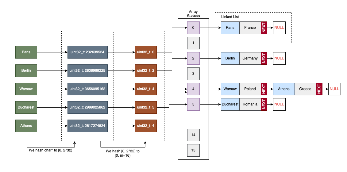
This is why hash table operations are average case $O(1)$. If the hash function is good and distributes keys evenly, the linked lists will be very short. In the unlikely worst case, where all keys collide into one bucket, the performance degrades to $O(n)$ as you'd have to search a single long linked list.

In C++, the std::unordered_map container is an implementation of a hash table. This is distinct from std::map, which is typically implemented as a self-balancing binary search tree (like a Red-Black Tree) and has $O(\log n)$ complexity for its operations.

The following graph clearly illustrates the performance difference for insertions as the number of elements grows. Notice how the time for unordered_map grows much more slowly than for map.

The Cherno provides a great C++-specific explanation of these two data structures.

Conclusion

In this lesson, we've moved from simply measuring complexity to strategically managing it. You've seen how making a deliberate trade-off—sacrificing some memory—can lead to significant gains in speed. This principle is at the heart of many advanced algorithms.

Key Takeaways:

• The time-space trade-off is a fundamental choice in algorithm design where you can often improve runtime performance at the cost of higher memory usage.
• Hash tables are a canonical example of this trade-off. They use extra space ($O(n)$) to provide fast, average-case constant-time ($O(1)$) lookups, insertions, and deletions.
• The Two Sum problem demonstrates this perfectly: a brute-force $O(n^2)$ time, $O(1)$ space solution can be optimized to an $O(n)$ time, $O(n)$ space solution using a hash table.
• In C++, std::unordered_map is your go-to for hash table functionality, offering superior performance over std::map when element ordering is not required.
• Articulating these trade-offs, justifying your choice of data structure, is a crucial skill for coding interviews.

In our next lesson, we will dive deeper into two of the most fundamental C++ Standard Template Library containers: vector and string. You'll learn how to use their APIs effectively to build solutions for common algorithmic problems.