Hello! Welcome to our next lesson in the Probability and Statistics module.
In our last session, we learned how to calculate and interpret the expected value () and variance () of random variables. These two numbers give us a powerful summary of a distribution's center and spread. You might recall seeing a table with standard formulas for the mean and variance of common distributions.
Today, we will bring that table to life. Our goal is to model scenarios using Bernoulli, Binomial, and Poisson distributions. These are three of the most fundamental discrete probability distributions you will encounter in data science and on the GATE exam. By the end of this 60-minute lesson, you will be able to:
- Identify the conditions under which each distribution is used.
- Apply their respective Probability Mass Functions (PMFs) to calculate probabilities.
- Use their standard formulas for mean and variance to analyze scenarios quickly.
- Simulate these distributions in Python using NumPy.
Let's begin by looking at the simplest of these: the Bernoulli distribution.
1. The Bernoulli Distribution: A Single Trial
A Bernoulli trial is the simplest possible random experiment: a single trial with only two possible outcomes. We typically label these outcomes as "success" (represented by 1) and "failure" (represented by 0).
Think of it as a single coin flip, a single free-throw attempt, or checking if a single manufactured part is defective.

The key parameter for a Bernoulli distribution is , the probability of success. The probability of failure is then .
To get a formal introduction, please watch the first part of the following video.
Bernoulli, Binomial and Poisson Random Variables
The video 'Bernoulli, Binomial and Poisson Random Variables' by slcmath@pc clearly defines the Bernoulli distribution and its properties.
Watch from the beginning until 04:42. Pay close attention to: The definition of a Bernoulli experiment. The parameter 'p'. The derivation of the mean (E(X) = p) and variance (Var(X) = pq). This directly builds on what we learned last lesson.
As the video explained, the key characteristics are:
- Random Variable : Number of successes, can only be 0 or 1.
- Parameter: (probability of success).
- PMF: and .
- Expected Value:
- Variance:
Simulating a Bernoulli Trial in Python
Given your interest in combining theory with code, let's see how to simulate this. We can use the numpy library, which is a cornerstone of data science in Python.
Seven Must-Know Statistical Distributions and Their ...
The article 'Seven Must-Know Statistical Distributions...' provides concise text summaries and simple Python code for simulation. Let's look at the section on the Bernoulli distribution.
Read the section '1, Bernoulli Distribution'. Focus on the assumptions and the Python simulation code using np.random.choice.
The code np.random.choice(['success','failure'], p=(0.9, 0.1)) is a straightforward way to simulate one trial where the probability of success is 0.9.
2. The Binomial Distribution: A Sequence of Trials
What happens when we perform more than one Bernoulli trial? For example, instead of one coin flip, we flip a coin 10 times. The Binomial distribution helps us model the number of successes in a fixed number of independent Bernoulli trials.
For a scenario to be modeled by a Binomial distribution, four conditions must be met:
- Fixed number of trials (n): We know exactly how many times the experiment is repeated (e.g., 10 coin flips).
- Two possible outcomes: Each trial is a success or a failure.
- Independent trials: The outcome of one trial does not affect the outcome of another.
- Constant probability of success (p): The probability of success is the same for every trial.
Understanding the Binomial Formula
The formula for the Binomial PMF can look intimidating, so let's build an intuition for it first.
Overexplaining the binomial distribution
The video 'Overexplaining the binomial distribution' from the Primer channel does a brilliant job of visually explaining where the binomial formula comes from.
Watch from the beginning until 09:02. The goal here is not to memorize every calculation, but to grasp the core ideas: How probabilities are multiplied for a sequence of events (e.g., Make-Miss-Make). Why the order of successes and failures doesn't change the probability of a specific sequence. Why we need to count the number of different ways a certain outcome (e.g., 7 successes in 10 trials) can happen. This counting part is the 'binomial coefficient'.
Now that you have the intuition, let's formalize it. The probability of getting exactly successes in trials is given by the Binomial PMF:
Where:
- is the binomial coefficient. It counts the number of ways to choose successes from trials.
- is the probability of getting successes.
- is the probability of getting failures.
The following video segment provides a concise formal explanation and connects it back to the mean and variance.
Bernoulli, Binomial and Poisson Random Variables
Let's return to the 'Bernoulli, Binomial and Poisson Random Variables' video for a formal summary and a worked example.
Watch from 04:42 to 18:42. Pay special attention to: The explanation of the PMF formula. The worked example of flipping a coin 10 times. The explanation that a Binomial variable is a sum of 'n' independent Bernoulli variables. This is the key to understanding why its mean and variance are simply n times the Bernoulli mean and variance.
This leads to the beautifully simple formulas for the mean and variance of a Binomial distribution:
- Expected Value:
- Variance:
Notice how these are just the mean and variance of a single Bernoulli trial, scaled by . This is because the trials are independent!
Simulating a Binomial Distribution in Python
We can easily simulate binomial experiments in Python.
Seven Must-Know Statistical Distributions and Their ...
The 'Seven Must-Know...' article also covers the Binomial distribution and its simulation.
Read section '2, Binomial Distribution'. Note the four assumptions and the Python code using np.random.binomial(n, p, size).
This function allows you to simulate thousands of binomial experiments in an instant, which is very useful for checking your understanding or modeling complex systems.
Test your understanding!
A student is taking a multiple-choice quiz with 10 questions. Each question has 4 options, and only one is correct. The student guesses randomly on every question.
- What distribution models the number of questions the student answers correctly? What are the values of its parameters?
- What is the probability that the student gets exactly 2 questions right? (You can leave the answer as an expression).
- What is the expected number of correct answers?
Show answer
-
This is a Binomial distribution because there's a fixed number of independent trials (10 questions) with a constant probability of success. The parameters are (number of trials) and (probability of guessing correctly on one question).
-
We want to find using the Binomial PMF:
There's about a 28% chance of getting exactly 2 questions right. -
The expected value is . On average, a student guessing randomly would get 2.5 questions correct.
3. The Poisson Distribution: Events over an Interval
Our final distribution for today is the Poisson distribution. While Binomial counts successes in a set number of trials, Poisson models the number of events occurring in a fixed interval of time or space.
Examples include:
- The number of emails you receive in an hour.
- The number of customers arriving at a store in a day.
- The number of typos on a page of a book.
The key parameter is (lambda), which is the average rate of events in that interval.
Bernoulli, Binomial and Poisson Random Variables
The final section of the slcmath@pc video explains the Poisson distribution.
Watch from 18:42 to the end (25:04). Focus on: The definition of a Poisson experiment (counting occurrences in a fixed interval). The parameter \lambda (the average). The PMF and the fact that both the mean and variance are equal to \lambda.
The core properties of the Poisson distribution are:
- Random Variable : Number of events, can be (theoretically infinite).
- Parameter: (average number of events per interval).
- PMF: , where is the number of events.
- Expected Value:
- Variance:
The Link Between Binomial and Poisson
The Poisson distribution can be seen as an approximation of the Binomial distribution when the number of trials is very large and the probability of success is very small. In this case, .
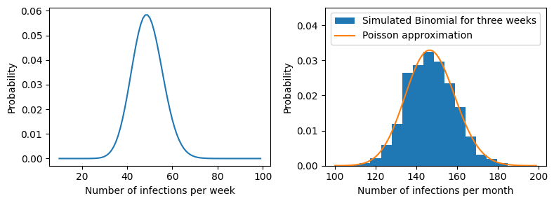
This connection is very useful and is a common topic in probability theory.
Seven Must-Know Statistical Distributions and Their ...
Let's read the final relevant sections of the two articles to solidify our understanding of Poisson and its connection to Binomial.
Read section '6, Poisson Distribution' and the summary section 'Relationships among Different Distributions'. This will reinforce the definition, provide the Python code np.random.poisson, and explicitly state the Binomial-Poisson relationship.
Test your understanding!
A call center receives an average of 5 calls per hour.
- What distribution models the number of calls received in any given hour? What is its parameter?
- What is the probability that the call center receives exactly 3 calls in a given hour?
- What is the probability of receiving 0 calls in an hour?
Show answer
-
This scenario is modeled by a Poisson distribution, as we are counting events (calls) over a fixed interval (an hour). The parameter is the average rate, .
-
We want to find using the Poisson PMF with :
There's about a 14% chance of receiving exactly 3 calls. -
We want to find :
There's a very small (less than 1%) chance of receiving zero calls in an hour. (Remember that ).
Conclusion
Excellent work today! We've covered three essential discrete distributions that form a major part of the probability syllabus for the GATE exam.
Key Takeaways:
Here is a summary table to help you keep these distributions straight:
| Feature | Bernoulli Distribution | Binomial Distribution | Poisson Distribution |
|---|---|---|---|
| Models | A single trial with two outcomes | Number of successes in independent trials | Number of events in a fixed interval |
| Parameters | (prob. of success) | (num. trials), (prob. of success) | (average rate of events) |
| PMF | |||
| Expected Value | |||
| Variance |
Understanding when to use each model is just as important as knowing the formulas. Always check the conditions of the scenario you are analyzing.
Preview of the Next Lesson:
Having covered the most important discrete distributions, we will now move to the continuous world. In our next lesson, we will model scenarios using Uniform, Exponential, and Normal distributions. The Normal distribution, in particular, is arguably the most important distribution in all of statistics and is fundamental to many machine learning concepts.