Hello! Welcome to our lesson on continuous probability distributions.
In our last session, we explored the world of discrete random variables, focusing on the Bernoulli, Binomial, and Poisson distributions. We saw how their Probability Mass Functions (PMFs) help us calculate the probability of specific, countable outcomes.
Today, we shift our focus to continuous random variables, which can take on any value within a given range. Think of measurements like height, weight, or time. Instead of a PMF, we will use a Probability Density Function (PDF). A key idea to grasp is that for a continuous variable, the probability of it being exactly one specific value is zero. Instead, we calculate the probability that the variable falls within an interval, which corresponds to the area under the PDF curve for that interval.
Our goal for this 60-minute lesson is to model scenarios using Uniform, Exponential, and Normal distributions. These are three of the most fundamental continuous distributions in data science and are essential for your GATE preparation.
By the end of this lesson, you will be able to:
- Identify which distribution best models a given continuous scenario.
- Understand the key properties (parameters, PDF, mean, variance) of each distribution.
- Use Python's
scipy.statslibrary to work with these distributions.
Let's begin with the simplest continuous distribution.
1. The Uniform Distribution: All Outcomes Equally Likely
Imagine you're waiting for a shuttle that arrives every 30 minutes. If you arrive at the stop at a random time, your waiting time could be any value between 0 and 30 minutes, and each of those times is equally likely. This is a classic scenario for a Continuous Uniform Distribution. It models a random variable where all outcomes within a specified range [a, b] have an equal chance of occurring.
The PDF is a flat line over the interval [a, b], which is why its graph looks like a rectangle. The height of this rectangle is to ensure the total area (total probability) is 1.
To see this in action and learn how to work with it in Python, please watch the first part of this video.
Python for Data Analysis: Probability Distributions
The video 'Python for Data Analysis: Probability Distributions' by DataDaft provides an excellent introduction to the uniform distribution and demonstrates its implementation in Python.
Watch from 01:11 to 06:56. Focus on: The flat shape of the uniform distribution's density plot. How to generate random numbers from a uniform distribution using stats.uniform.rvs(). The meaning and use of the .cdf() (Cumulative Distribution Function) and .ppf() (Percent Point Function, the inverse of CDF) functions.
As the video explained, the scipy.stats library is your primary tool for this. Let's summarize the key properties:
- Scenario: Any situation where outcomes in a range are equally likely.
- Parameters:
a(minimum value,locinscipy) andb(maximum value,loc + scaleinscipy). - PDF: for , and 0 otherwise.
- Expected Value: (the midpoint of the interval).
- Variance: .
For more details on the Python implementation, you can refer to the following article.
Probability Distributions in Python Tutorial
For a quick text reference and code example, the DataCamp tutorial 'Probability Distributions in Python' is very helpful.
Read the section 'Uniform Distribution Function'. Note how the loc and scale parameters in scipy.stats.uniform map to a and b-a.
2. The Exponential Distribution: Waiting Time Between Events
In our last lesson, we used the Poisson distribution to model the number of events in an interval (e.g., 5 customers arriving per hour). The Exponential Distribution is its natural partner: it models the time between those events. It's used to describe the waiting time until the next event in a process where events happen independently and at a constant average rate.
Examples include:
- The time until the next customer calls a support center.
- The time until a radioactive particle decays.
- The lifespan of a component that fails at a constant rate.
A key property of the exponential distribution is that it is memoryless. This means that if a component has already lasted for 100 hours, the probability that it lasts for another 50 hours is the same as the probability that a brand-new component lasts for 50 hours.
Let's watch a short video segment that introduces this distribution.
Python for Data Analysis: Probability Distributions
Returning to the DataDaft video, let's look at the segment on the exponential distribution.
Watch from 27:06 to 28:47. Observe the shape of the distribution: it's most likely that the waiting time will be short, and very long waiting times are rare.
The distribution is defined by a single parameter, (lambda), the average rate of events.
- Scenario: Waiting time between events in a Poisson process.
- Parameter: The rate parameter (e.g., 5 customers/hour).
- PDF: for .
- Expected Value: . This is intuitive: if the rate is 5 customers/hour, the average time between customers is 1/5 of an hour.
- Variance: .
Important note on Python implementation: In scipy.stats.expon, the scale parameter is used, which is equal to . So, if the rate is 5, you would set scale=1/5.
Seven Must-Know Statistical Distributions and Their ...
The article 'Seven Must-Know Statistical Distributions...' gives a great explanation of how the Exponential distribution is derived from the Poisson process, which directly connects to our previous lesson.
Read section '7, Exponential Distribution'. Pay close attention to the derivation from the Poisson CDF, and the formulas for expected value and variance in terms of \lambda.
Test your understanding!
A factory produces light bulbs. On average, 2 bulbs per 1000 hours of operation are found to be defective. A quality inspector picks a new bulb and tests it.
- What distribution would you use to model the time (in hours) until this new bulb becomes defective?
- What is the value of the rate parameter ?
- What is the expected time until the bulb fails?
Show answer
- This is a waiting time problem with a constant average rate of failure, so we use the Exponential Distribution.
- The rate of failure is failures per hour.
- The expected time to failure is hours.
3. The Normal Distribution: The Bell Curve
The Normal (or Gaussian) Distribution is arguably the most important distribution in all of statistics. It's found everywhere, describing phenomena in both nature and society. This is partly due to the Central Limit Theorem, a powerful idea stating that if you take many random samples and average them, the distribution of those averages will tend to be normal, regardless of the original distribution.
Examples of things that are often normally distributed:
- Heights and weights of a population.
- Measurement errors in an experiment.
- IQ scores.
- Blood pressure.
It is defined by two parameters: the mean , which is the center of the distribution, and the standard deviation , which determines its spread.
Normal Distribution EXPLAINED with Examples
The video 'Normal Distribution EXPLAINED with Examples' from Ace Tutors gives a fantastic high-level explanation of the Normal distribution, the 68-95-99.7 rule, and the concept of standardization.
Watch from the beginning to 03:50, and then from 05:37 to 10:26. Don't worry about memorizing the Z-chart details; focus on: The bell shape and its symmetry around the mean \mu. The Empirical Rule: about 68% of data is within \pm 1\sigma, 95% within \pm 2\sigma, and 99.7% within \pm 3\sigma. Why we standardize data and what a Z-score represents (number of standard deviations from the mean). The logic used in the pizza example to find probabilities for 'less than', 'greater than', and 'between' scenarios.
Standardization and the Z-score
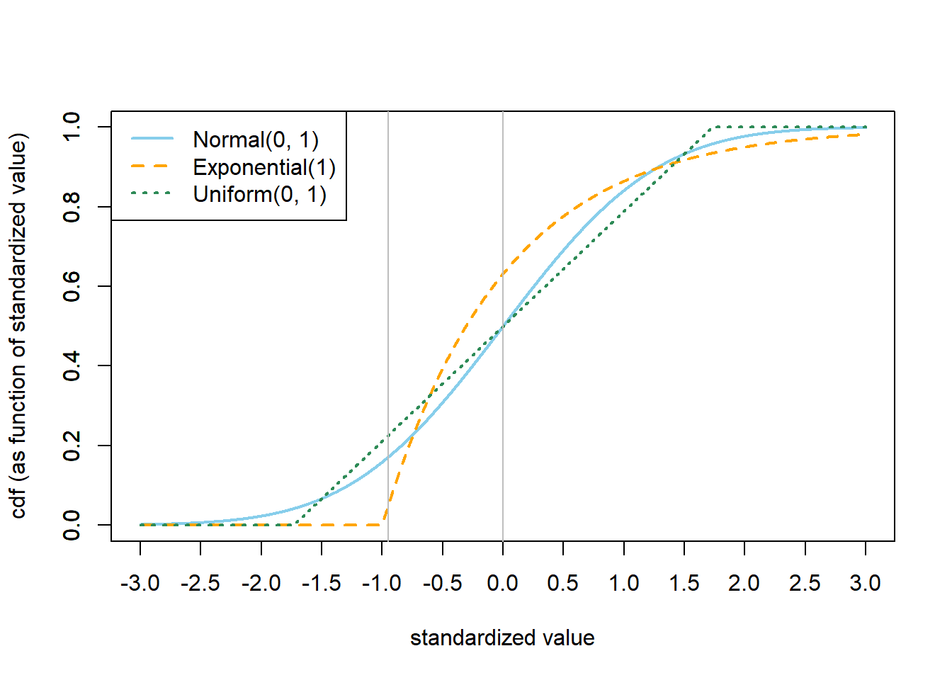
As the video explained, a crucial concept is standardization. To compare different normal distributions (e.g., pizza sizes vs. student heights), we convert them to a Standard Normal Distribution, which has a mean of 0 and a standard deviation of 1. We do this by calculating a Z-score:
The Z-score tells us exactly how many standard deviations an observation is from the mean .
Working with the Normal Distribution in Python
While Z-tables were traditionally used, Python makes finding these probabilities much easier. Let's see how scipy handles this.
Python for Data Analysis: Probability Distributions
The DataDaft video shows how to apply these concepts in Python, using the same functions we saw for the uniform distribution.
Watch from 12:06 to 16:45. Pay close attention to how stats.norm.ppf() is used to find a cutoff value for a given probability (like the bottom 2.5%) and how stats.norm.cdf() is used to find the cumulative probability up to a certain value.
Let's recap the key properties:
- Scenario: Describes many natural phenomena; distribution of sample means.
- Parameters: Mean (
locinscipy) and standard deviation (scaleinscipy). - PDF: A symmetric, bell-shaped curve centered at .
- Expected Value: .
- Variance: .
Test your understanding!
The scores on a standardized test are normally distributed with a mean and a standard deviation .
- What is the Z-score for a student who scored 130?
- Using the Empirical Rule, approximately what percentage of students score between 85 and 115?
- Would you expect a score of 150 to be common or rare? Why?
Show answer
- The Z-score is . This means a score of 130 is exactly 2 standard deviations above the mean.
- The range from 85 to 115 is exactly one standard deviation below the mean () to one standard deviation above the mean (). According to the Empirical Rule, approximately 68% of students score in this range.
- A score of 150 would be very rare. Its Z-score is . This is more than 3 standard deviations from the mean. The Empirical Rule tells us that 99.7% of all scores fall within 3 standard deviations, so a score beyond that is highly unlikely.
Conclusion
Great job! Today you've learned about three essential continuous distributions that are cornerstones of probability and statistics.
Key Takeaways:
Here is a summary table to help you distinguish between them:
| Feature | Uniform Distribution | Exponential Distribution | Normal Distribution |
|---|---|---|---|
| Models | All outcomes in a range are equally likely | Time between events in a Poisson process | Many natural phenomena; bell-shaped data |
| Parameters | a (min), b (max) |
λ (rate) |
μ (mean), σ (std. dev.) |
| PDF Shape | Rectangle | Decreasing curve | Symmetrical Bell Curve |
| Expected Value | |||
| Variance |
The most important skill is recognizing which distribution to apply to a problem. Always think about what the random variable represents: a value from an equally likely range (Uniform), a waiting time (Exponential), or a measurement that clusters around an average (Normal).
Preview of the Next Lesson:
We've now covered the theoretical foundations of the most common probability distributions. In our next lesson, we will get our hands dirty with real data. You will learn how to compute and interpret descriptive statistics (mean, median, variance) for a dataset using Pandas. This will bridge the gap between theoretical probability and practical data analysis.