Expected Value and Variance of Random Variables

1. Expected Value: The Center of a Distribution

The expected value of a random variable is its theoretical mean. Imagine repeating an experiment an infinite number of times and averaging the outcomes; that average would be the expected value. It's the "center of mass" of the probability distribution. We denote it as $E(X)$ or by the Greek letter $\mu$ (mu).

Expected Value of a Discrete Random Variable

For a discrete random variable, the expected value is a weighted average of all possible values, where each value is weighted by its probability.

The formula is:
$E(X)=\mu ={\sum }_{\text{all }x}x\cdot P(X=x)$

Here, you take each possible value $x$, multiply it by the probability of that value occurring, and sum up all these products.

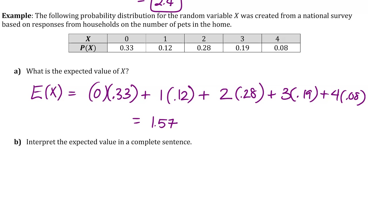
To see a detailed walkthrough of this concept, let's watch the first part of a helpful video.

An important point from the video is that the expected value might not be a value that the random variable can actually take. For instance, in the image example, $E(X)=1.57$, but you can't own 1.57 pets. It's the long-term average.

Expected Value of a Continuous Random Variable

For continuous random variables, the logic is the same, but we replace the summation with an integral. Since probability is the area under the PDF curve, we integrate the product of the value $x$ and the probability density $f(x)$ over the entire range of possible values.

The formula is:
$E(X)=\mu ={\int }_{-\infty }^{\infty }x\cdot f(x)dx$

Let's watch a video that brilliantly visualizes how the discrete sum naturally becomes an integral as we move to continuous variables.

To see this formula in action, let's look at a text resource that works through some standard examples.

2. Variance and Standard Deviation: The Spread of a Distribution

While expected value tells us about the center of a distribution, it doesn't tell us how spread out the values are. For that, we use variance and standard deviation.

Variance, denoted $Var(X)$ or ${\sigma }^2$, is the expected value of the squared difference from the mean. A small variance means the data points tend to be very close to the mean; a large variance means they are spread out.

Standard Deviation, denoted $\sigma$, is simply the square root of the variance. Its advantage is that it is in the same units as the random variable, making it more interpretable.

Variance of a Discrete Random Variable

There are two common formulas for variance:

1. The Definitional Formula: This is good for interpretation.
   $Var(X)={\sigma }^2=E[(X-\mu {)}^2]={\sum }_{\text{all }x}(x-\mu {)}^2\cdot P(X=x)$
2. The Computational Formula: This is usually easier for calculations.
   $Var(X)={\sigma }^2=E[X^2]-(E[X]{)}^2=E[X^2]-{\mu }^2$
   To use this, you first calculate $E[X^2]=\sum x^2\cdot P(X=x)$, and then subtract the square of the mean (${\mu }^2$) which you already calculated.

Let's see how both of these formulas are used in practice.

Variance of a Continuous Random Variable

The formulas for continuous variables are analogous, with integrals replacing sums:

1. The Definitional Formula:
   $Var(X)={\sigma }^2={\int }_{-\infty }^{\infty }(x-\mu {)}^2\cdot f(x)dx$
2. The Computational Formula:
   $Var(X)={\sigma }^2=E[X^2]-{\mu }^2=\left({\int }_{-\infty }^{\infty }{x}^2\cdot f(x)dx\right)-{\mu }^2$

The following resource formally defines these and provides key examples.

3. Properties and Shortcuts

For the GATE exam, knowing some key properties and standard formulas will save you a lot of time.

Properties of Expectation and Variance

Let $X$ be a random variable and $a,b$ be constants.

1. $E(aX+b)=aE(X)+b$
   • Interpretation: If you scale a variable by $a$ and shift it by $b$, the mean is also scaled and shifted.
2. $Var(aX+b)=a^{2}Var(X)$
   • Interpretation: Shifting a distribution ($+b$) doesn't change its spread. Scaling it by $a$ multiplies the variance by $a^2$ (and the standard deviation by $|a|$).

Formulas for Common Distributions

For many standard distributions you will encounter, the expected value and variance are given by simple formulas. Memorizing these is crucial for efficiency.

Conclusion

Great work! You've now learned how to distill a potentially complex probability distribution into two simple, meaningful numbers: its center and its spread.

Key Takeaways:

• Expected Value ($\mu$) is the long-run average or "center of mass" of a random variable.
  • Discrete: $E(X)=\sum x\cdot P(X=x)$
  • Continuous: $E(X)=\int x\cdot f(x)dx$
• Variance (${\sigma }^2$) measures the expected squared deviation from the mean, quantifying the "spread" of the distribution.
  • The computational formula is often easiest: $Var(X)=E[X^2]-(E[X]{)}^2$.
• Standard Deviation ($\sigma$) is the square root of the variance and has the same units as the random variable, making it easy to interpret.
• Knowing the properties of $E(X)$ and $Var(X)$, along with the standard formulas for common distributions, is a critical skill for problem-solving.

Preview of the Next Lesson:

In this lesson, we saw a table of formulas for common distributions. In our next session, we'll dive deep into some of these, starting with discrete distributions. We will model scenarios using the Bernoulli, Binomial, and Poisson distributions, learning when to use each one and how to solve problems with them.