Dimensionality Reduction with PCA

1. The Intuition Behind PCA

Imagine you have a dataset with many features. PCA's goal is to create a new, smaller set of features that are combinations of the original ones. These new features, called principal components, are carefully constructed to be uncorrelated and to capture the maximum possible information, or variance, from the original data.

Let's start by building a strong visual intuition for this process.

As the video explains, PCA finds the directions in your data where the points are most spread out.

• The first principal component (PC1) is the direction (or axis) that captures the largest amount of variance.
• The second principal component (PC2) is the next direction that captures the most remaining variance, with the condition that it must be orthogonal (perpendicular) to PC1.
• This continues for all dimensions.

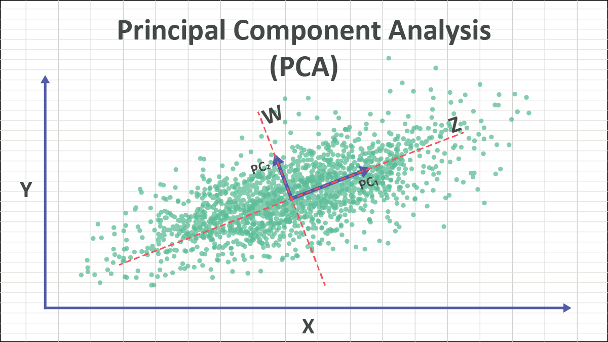
By transforming the data onto this new coordinate system, we can often discard the later principal components (which capture very little variance) and represent our data in a lower-dimensional space with minimal information loss.

2. How PCA Works: The Step-by-Step Process

Now that we have the intuition, let's walk through the steps involved. We'll combine a high-level conceptual guide with a look at the underlying mathematics. You've already covered the necessary linear algebra concepts like covariance, eigenvectors, and eigenvalues, so you'll see how they are practically applied here.

We can break down PCA into five main steps.

Here is a summary of those five steps, with some added detail:

1. Standardize the Data: Just like with K-Means, PCA is sensitive to the scale of the original variables. If one feature has a much larger range than others, it will dominate the analysis. Therefore, we must first standardize our data (e.g., by transforming it to have a mean of 0 and a standard deviation of 1). The StatQuest video referred to this as "centering" the data.

2. Compute the Covariance Matrix: The covariance matrix tells us how every variable in our dataset relates to every other variable. The diagonal elements are the variances of each variable, and the off-diagonal elements are the covariances between pairs of variables. This matrix is fundamental because it quantifies the "spread" of our data.

3. Compute Eigenvectors and Eigenvalues: This is the core mathematical step of PCA. We perform an eigen decomposition of the covariance matrix.

   • The eigenvectors of the covariance matrix point in the directions of maximum variance. These are our principal components!
   • The eigenvalues tell us the amount of variance captured by each corresponding eigenvector (i.e., each principal component).

4. Create a Feature Vector (Select Principal Components): We sort the eigenvalues in descending order. The eigenvector with the highest eigenvalue is the first principal component (PC1), as it captures the most variance. We then decide how many principal components we want to keep. For dimensionality reduction, we would choose to keep the first $k$ eigenvectors, where $k$ is smaller than the original number of dimensions.

5. Project Data onto the New Axes: Finally, we use the feature vector (the matrix of the top eigenvectors we decided to keep) to transform our original standardized data into the new, lower-dimensional space. This new dataset consists of the principal component scores.

The Math in Action

To see how the covariance matrix and its eigenvectors/eigenvalues produce the principal components, let's look at a mathematical walkthrough.

The most important takeaway from this is that the eigenvalues of the covariance matrix are the variances of the principal components. This property is what allows us to quantify exactly how much information each principal component holds.

3. Applying PCA in Python

Theory is great, but let's see how to apply PCA for dimensionality reduction in code. We'll use scikit-learn, which makes this process very straightforward.

Let's summarize the workflow in scikit-learn:

import numpy as np
from sklearn.decomposition import PCA
from sklearn.preprocessing import StandardScaler

# Assume 'X' is your original data with shape (n_samples, n_features)
# For example, 150 samples and 10 features
X = np.random.rand(150, 10)

# 1. Standardize the data
scaler = StandardScaler()
X_scaled = scaler.fit_transform(X)

# 2. Initialize PCA
# Let's say we want to reduce to 2 dimensions
pca = PCA(n_components=2)

# 3. Fit and transform the data
X_pca = pca.fit_transform(X_scaled)

# Now X_pca is our new, lower-dimensional data
print("Original shape:", X_scaled.shape)
print("Transformed shape:", X_pca.shape)

# You can inspect the explained variance
print("Explained variance ratio:", pca.explained_variance_ratio_)

The explained_variance_ratio_ attribute shows the proportion of the dataset's variance that lies along each principal component. In our example, [0.15, 0.12] would mean PC1 accounts for 15% of the variance and PC2 accounts for 12%.

Choosing the Number of Components

So, how do we choose the right number of components, like n_components=2? We don't want to pick an arbitrary number. The goal is to keep enough components to preserve most of the data's information while still achieving a meaningful reduction in dimensionality.

We can do this by looking at the cumulative explained variance. We plot the total variance explained as we add more and more principal components. This plot is often called a scree plot.

The typical goal is to choose a number of components that captures a high percentage of the total variance, often between 90% and 99%. The plot helps you see the trade-off. For example, you might find that you need 20 components to explain 95% of the variance in a 100-dimensional dataset. This would be a reduction from 100 features to just 20, which is a huge improvement!

Conclusion

Great work! You've just learned about one of the most widely used techniques in data science and machine learning. PCA is not only for visualization but is also a common preprocessing step to improve the speed and performance of other machine learning algorithms.

Key Takeaways:

• Principal Component Analysis (PCA) is an unsupervised learning method used for dimensionality reduction.
• It works by finding a new set of axes—principal components—that are orthogonal and aligned with the directions of maximum variance in the data.
• The process involves standardizing the data, computing the covariance matrix, and then finding its eigenvectors (the PCs) and eigenvalues (the variance explained by each PC).
• The effectiveness of PCA is measured by the cumulative explained variance, which helps you decide how many components to keep to preserve a desired amount of information (e.g., 95%).
• scikit-learn provides a simple and powerful implementation through the PCA class.

Preview of the Next Lesson:
So far, we've learned to apply individual steps like feature scaling (in K-Means) and dimensionality reduction (with PCA) before training a model. In a real project, you might chain many such steps together. In the next lesson, we will learn how to build a complete modeling workflow using scikit-learn's Pipeline object. This will allow you to cleanly combine preprocessing steps and a final estimator into a single, elegant object.