Finding Local Extrema with Derivative Tests

1. What are Maxima and Minima?

When we look at the graph of a function, we can often visually identify its highest and lowest points. In calculus, we give these points specific names:

• A local maximum is a point that is higher than all of its immediate neighbors. Think of it as the peak of a small hill.
• A local minimum is a point that is lower than all of its immediate neighbors. Think of it as the bottom of a small valley.
• A global (or absolute) maximum/minimum is the absolute highest or lowest point across the function's entire domain or a specified interval.

A function can have multiple local maxima and minima, but only one global maximum and one global minimum within a given interval.

To get a clear visual understanding of these concepts, let's watch a short video segment.

2. Finding Potential Maxima and Minima: Stationary Points

How can we find these peaks and valleys without looking at a graph? The key lies in the derivative.

Think about standing at the very top of a hill (a maximum) or the very bottom of a valley (a minimum). At that exact point, the ground is flat. The slope is zero. In calculus terms, this means the first derivative of the function is zero.

Points where the first derivative, $f^{\prime }(x)$, is equal to zero are called stationary points or critical points. These are our candidates for being local maxima or minima.

The procedure is:

1. Given a function $f(x)$.
2. Find its first derivative, $f^{\prime }(x)$.
3. Set the derivative to zero: $f^{\prime }(x)=0$.
4. Solve this equation for $x$. The solutions are your stationary points.

Let's watch a quick example of finding these stationary points.

Once we have a stationary point, we need to determine if it's a maximum, a minimum, or something else. We have two main tools for this: the First Derivative Test and the Second Derivative Test.

3. The First Derivative Test

The first derivative doesn't just tell us where the slope is zero; its sign tells us if the function is increasing or decreasing.

• If $f^{\prime }(x)>0$, the function is increasing.
• If $f^{\prime }(x)<0$, the function is decreasing.

We can use this to classify our stationary points. Imagine moving along the x-axis and passing through a stationary point c:

• If the function was increasing ($f^{\prime }>0$) and then becomes decreasing ($f^{\prime }<0$), you must have gone over a peak. So, c is a local maximum.
• If the function was decreasing ($f^{\prime }<0$) and then becomes increasing ($f^{\prime }>0$), you must have passed through a valley. So, c is a local minimum.

The following video segment explains this test and introduces a very useful technique called the "wavy curve method" for applying it, which is particularly handy for the polynomial functions you'll often see in the GATE exam.

4. The Second Derivative Test: A More Direct Approach

Checking the sign of the first derivative on both sides of a point can sometimes be tedious. The Second Derivative Test is often a faster way to classify stationary points.

The second derivative, $f^{\prime \prime }(x)$, tells us about the function's concavity.

• If $f^{\prime \prime }(x)>0$, the function is concave up (shaped like a cup, U).
• If $f^{\prime \prime }(x)<0$, the function is concave down (shaped like a frown, ∩).

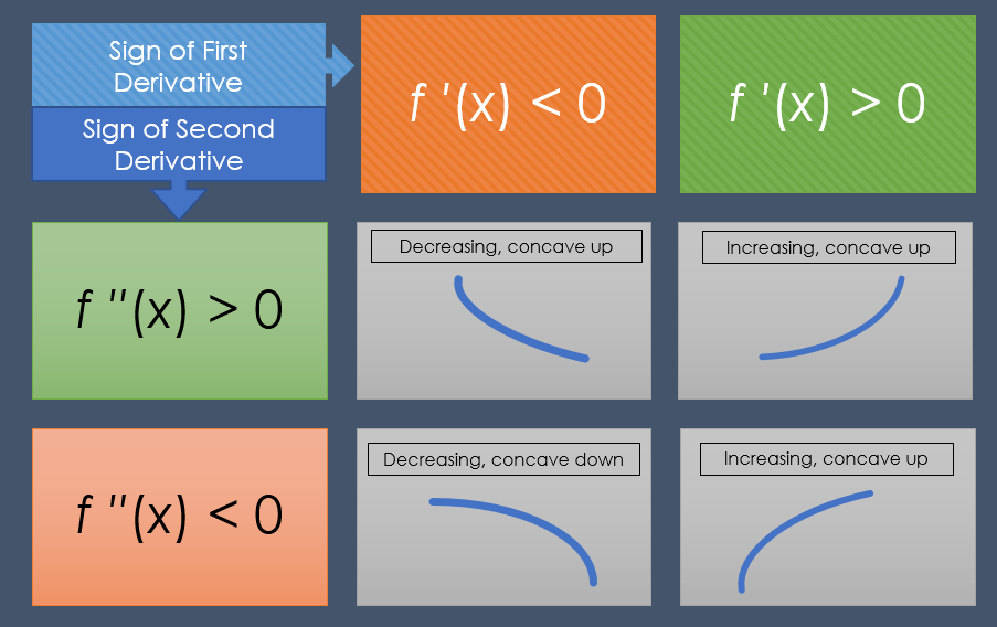
Now, let's connect this to our stationary points. If we are at a stationary point (where $f^{\prime }(x)=0$):

• If the function is concave down ($f^{\prime \prime }(x)<0$), the point must be a local maximum.
• If the function is concave up ($f^{\prime \prime }(x)>0$), the point must be a local minimum.

The Second Derivative Test Procedure:

1. Find the stationary points by solving $f^{\prime }(x)=0$.
2. Find the second derivative, $f^{\prime \prime }(x)$.
3. For each stationary point $c$, evaluate $f^{\prime \prime }(c)$.
   • If $f^{\prime \prime }(c)<0$, then $x=c$ is a local maximum.
   • If $f^{\prime \prime }(c)>0$, then $x=c$ is a local minimum.
   • If $f^{\prime \prime }(c)=0$, the test is inconclusive. You must use the First Derivative Test instead.

The case where $f^{\prime \prime }(x)=0$ might indicate a point of inflection, where the concavity changes but there is no maximum or minimum (e.g., the point $x=0$ for the function $f(x)=x^3$).

To understand the logic behind the second derivative test, watch this short, clear explanation.

5. Finding Absolute Maxima and Minima in a Closed Interval

A very common type of problem in GATE and other exams is to find the absolute maximum and minimum values of a function on a closed interval, like $[a,b]$.

The absolute extremum can occur either at one of the local extrema inside the interval or at the endpoints of the interval ($x=a$ or $x=b$).

Procedure to find absolute extrema on $[a,b]$:

1. Find all stationary points of $f(x)$ that lie within the interval $(a,b)$.
2. Make a list of candidate points: the stationary points from step 1, and the two endpoints $a$ and $b$.
3. Evaluate the function $f(x)$ at every candidate point in your list.
4. The largest value you find is the absolute maximum, and the smallest is the absolute minimum.

This method is foolproof. You don't even need the second derivative test here; you just compare the function values at the end.

Conclusion

Great job today! You've mastered a crucial piece of calculus that forms the bedrock of optimization theory.

Key Takeaways:

• Stationary points, where $f^{\prime }(x)=0$, are the candidates for local maxima or minima.
• The First Derivative Test checks the sign of $f^{\prime }(x)$ around a stationary point to classify it (positive to negative = max; negative to positive = min).
• The Second Derivative Test uses the sign of $f^{\prime \prime }(x)$ at a stationary point for a more direct classification ($f^{\prime \prime }<0$ = max; $f^{\prime \prime }>0$ = min).
• To find the absolute maximum/minimum on a closed interval $[a,b]$, you must check the value of $f(x)$ at both the internal stationary points and the endpoints $a$ and $b$.

Preview of the Next Lesson:

Now that we are experts at finding the minimum of a one-dimensional function, we are ready to return to the multivariable world. In the next lesson, we will learn about gradient descent. This is the core algorithm used to train most machine learning models. It uses the gradient we learned about last lesson to iteratively "walk" down the surface of a high-dimensional cost function, taking steps in the direction of steepest descent to find a minimum, just as we did today using derivative tests.