Partial Derivatives and Gradients

Hello! Welcome to your third lesson on Calculus for Optimization.

In our last lesson, we mastered the product, quotient, and chain rules, which gave us the power to differentiate almost any single-variable function. We saw that the derivative $\frac{df}{d x}$ measures the rate of change of a function $f (x)$ as its single input $x$ changes.

However, in data science and machine learning, functions rarely have just one input. Think of a model predicting a house price: its inputs could be square footage, number of bedrooms, and distance from the city center. The model's error, or "cost," is a function of all these variables. To optimize the model, we need to know how the cost changes as we tweak each of these variables. This requires moving from single-variable calculus to multivariable calculus.

Today's lesson is our first step into this new world. Our learning outcome is to compute partial derivatives and gradients of multivariable functions. This is a fundamental skill for understanding how machine learning models are trained.

1. The Need for a New Kind of Derivative

When a function has only one input, $f (x)$ , there's only one "direction" it can change: along the x-axis. But for a function with two inputs, $f (x, y)$ , the input is a point on a 2D plane. From any point, you can move in an infinite number of directions. Does the function's value increase faster if you move along the x-axis, the y-axis, or somewhere in between?

This ambiguity means we can't have a single "derivative." Instead, we introduce partial derivatives.

A partial derivative measures the rate of change of a multivariable function with respect to one input variable, while treating all other input variables as if they were constants.

To get a feel for this idea, let's watch a video that explains why we need to think about derivatives differently for functions of multiple variables.

Geometrical Meaning | Partial Derivative of Multivariate Functions | Machine Learning Uses | GATE DA

This video from GO Classes for GATE DA introduces the concept of multivariable functions and explains why the familiar single-variable derivative is not sufficient for them. This channel is specifically aimed at GATE DA preparation, making it highly relevant to your goal.

Watch the first part of the video, from the beginning to 12:28. Focus on the core problem: with multiple input variables, there are multiple directions of change, so we need a way to specify which direction we're interested in.

2. Computing Partial Derivatives

The notation for a partial derivative uses a curly "d" symbol, $\partial$ , called "del."

The partial derivative of $f$ with respect to $x$ is written as $\frac{\partial f}{\partial x}$ or $f_{x}$ .
The partial derivative of $f$ with respect to $y$ is written as $\frac{\partial f}{\partial y}$ or $f_{y}$ .

The key to computing a partial derivative is simple: when differentiating with respect to one variable, treat all other variables as constants.

Let's see this in action. Suppose we have the function:
$f (x, y) = x^{2} y^{3} + 2 x + 5 y$

To find $\frac{\partial f}{\partial x}$ :
We treat $y$ as a constant. Think of $y^{3}$ as just some number.

The derivative of $x^{2} y^{3}$ with respect to $x$ is $(y^{3}) \cdot (2 x) = 2 x y^{3}$ .
The derivative of $2 x$ with respect to $x$ is $2$ .
The derivative of $5 y$ with respect to $x$ is $0$ , because we're treating $y$ as a constant.
So, $\frac{\partial f}{\partial x} = 2 x y^{3} + 2$ .

To find $\frac{\partial f}{\partial y}$ :
We treat $x$ as a constant. Think of $x^{2}$ as just some number.

The derivative of $x^{2} y^{3}$ with respect to $y$ is $(x^{2}) \cdot (3 y^{2}) = 3 x^{2} y^{2}$ .
The derivative of $2 x$ with respect to $y$ is $0$ .
The derivative of $5 y$ with respect to $y$ is $5$ .
So, $\frac{\partial f}{\partial y} = 3 x^{2} y^{2} + 5$ .

For a quick and clear summary of this process, watch the following short clip.

Partial Derivatives and the Gradient of a Function

This clip from the 'Professor Dave Explains' channel provides a concise walkthrough of how to compute partial derivatives by treating other variables as constants.

Watch from 02:30 to 05:17. This segment clearly explains the notation and demonstrates the computation with a straightforward example.

Graphical Interpretation

What does a partial derivative look like? Imagine the graph of $f (x, y)$ as a 3D surface.

Multivariable Calculus: Partial Derivatives Visualized — This image shows the graph of a function $f(x, y)$ as a surface. When we calculate $\frac{\partial f}{\partial x}$, we are essentially slicing this surface with a plane where $y$ is held constant (the blue plane). The partial derivative is the slope of the tangent line to the curve created by this slice.

To solidify this, the following article provides an excellent explanation.

Introduction to partial derivatives (article)

This article from Khan Academy, 'Introduction to partial derivatives', gives a detailed yet intuitive explanation of what partial derivatives are and how to interpret them graphically.

Read the sections 'Example: Computing a partial derivative', 'Interpreting partial derivatives with graphs', and 'A more formal definition'. This will reinforce how to compute partial derivatives and connect the math to the graphical idea of slicing a surface.

Test your understanding!

Consider the function $f (x, y) = e^{x} cos (y)$ . Find the partial derivatives $\frac{\partial f}{\partial x}$ and $\frac{\partial f}{\partial y}$ .

Show answer

To find $\frac{\partial f}{\partial x}$ , treat $cos (y)$ as a constant. The derivative of $e^{x}$ is $e^{x}$ .
$\frac{\partial f}{\partial x} = e^{x} cos (y)$

To find $\frac{\partial f}{\partial y}$ , treat $e^{x}$ as a constant. The derivative of $cos (y)$ is $- sin (y)$ .
$\frac{\partial f}{\partial y} = e^{x} (- sin (y)) = - e^{x} sin (y)$

3. The Gradient: Combining Partial Derivatives

We now have two partial derivatives for our function $f (x, y)$ , one for the x-direction and one for the y-direction. It's useful to package this information into a single object: a vector. This vector is called the gradient.

The gradient of a function $f$ , denoted by $\nabla f$ (read "del f" or "grad f"), is the vector of all its partial derivatives. For a two-variable function $f (x, y)$ , the gradient is:

$\nabla f (x, y) = [\frac{\partial f}{\partial x} \frac{\partial f}{\partial y}] = ⟨ \frac{\partial f}{\partial x}, \frac{\partial f}{\partial y} ⟩$

The gradient is incredibly important in machine learning for one key reason:

The gradient vector $\nabla f$ at a point $(x_{0}, y_{0})$ points in the direction of the steepest ascent of the function $f$ at that point.

This means if you want to increase the function's value as quickly as possible, you should move in the direction of the gradient. Conversely, to decrease it as quickly as possible, you move in the opposite direction of the gradient. This is the core idea behind gradient descent, which we will explore soon.

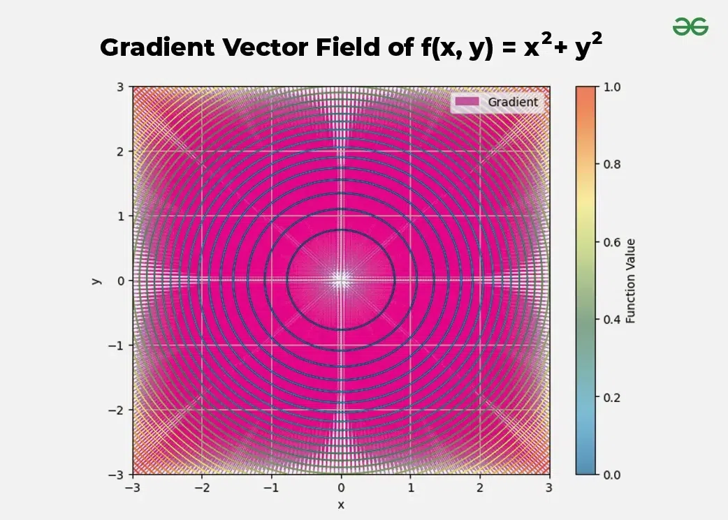
Gradient Vector Field of f(x, y) = x + y — This image shows the gradient field for the function $f(x,y) = x^2 + y^2$. The arrows (gradient vectors) point outwards, away from the center minimum. This is the direction of the steepest increase at each point.

Let's see how to compute and interpret the gradient.

The gradient vector | Multivariable calculus (article)

This Khan Academy article, 'The gradient vector', formally defines the gradient and explains its significance.

Read the sections 'Definition' and 'Example 1: Two dimensions'. Focus on how the gradient is constructed from the partial derivatives you just learned to compute.

Example:
For our earlier function $f (x, y) = x^{2} y^{3} + 2 x + 5 y$ , we found:

$\frac{\partial f}{\partial x} = 2 x y^{3} + 2$
$\frac{\partial f}{\partial y} = 3 x^{2} y^{2} + 5$

The gradient of this function is the vector:
$\nabla f (x, y) = [2 x y^{3} + 2 3 x^{2} y^{2} + 5]$

4. The Chain Rule for Multivariable Functions

In the previous lesson, we learned the chain rule for nested single-variable functions. This rule also extends to multivariable calculus and is the mathematical foundation for backpropagation, the algorithm used to train neural networks.

Imagine a function $z = f (x, y)$ , but $x$ and $y$ themselves depend on another variable, say $t$ . For example, $x = g (t)$ and $y = h (t)$ . Ultimately, $z$ is a function of a single variable, $t$ . How do we find $\frac{d z}{d t}$ ?

We can visualize the dependencies using a tree diagram:

$z$ depends on $x$ and $y$ .
$x$ and $y$ both depend on $t$ .

To find the total rate of change of $z$ with respect to $t$ , we sum the contributions from all paths leading from $z$ to $t$ :
$\frac{d z}{d t} = \frac{\partial z}{\partial x} \frac{d x}{d t} + \frac{\partial z}{\partial y} \frac{d y}{d t}$
Notice the mix of partial ( $\partial$ ) and total ( $d$ ) derivative symbols. We use $\partial$ when a variable depends on multiple others, and $d$ when it depends on only one.

The video below explains this rule and explicitly connects it to its importance in machine learning.

Geometrical Meaning | Partial Derivative of Multivariate Functions | Machine Learning Uses | GATE DA

Let's return to the GO Classes video. The second half explains the multivariable chain rule, which is critical for understanding backpropagation in neural networks.

Watch from 51:19 to 57:55. Focus on the tree diagram and how it helps construct the chain rule formula. Note the connection made to backpropagation, which is a key concept you'll encounter later in your studies.

Conclusion

Excellent work! You've successfully taken your first major step into multivariable calculus, a cornerstone of modern data science and AI.

Key Takeaways:

A partial derivative ( $\frac{\partial f}{\partial x}$ ) measures the rate of change of a multivariable function along one axis, treating other variables as constants.
The gradient ( $\nabla f$ ) is a vector that bundles all partial derivatives together.
The gradient vector points in the direction of the steepest increase of the function. This property is what makes it the engine of optimization algorithms.
The multivariable chain rule allows us to calculate derivatives through nested dependencies and is the basis for the backpropagation algorithm in deep learning.

Preview of the Next Lesson:

The gradient tells us the direction to move to minimize a function, but it doesn't tell us how far to move. Before we dive into the gradient descent algorithm, we'll first solidify our understanding of optimization in a simpler context. In the next lesson, we will revisit single-variable functions and learn how to use derivatives to find their local maxima and minima. This will build the final piece of intuition we need before tackling optimization in multiple dimensions.