Understanding Gradient Descent

1. The Core Idea: Walking Downhill

Imagine you are standing on a hilly landscape in thick fog and you want to get to the lowest point. You can't see the whole landscape, but you can feel the steepness of the ground right where you are. What's the best strategy?

You would probably:

1. Feel the ground to find the direction of the steepest slope downhill.
2. Take a small step in that direction.
3. Repeat the process.

This is the exact intuition behind gradient descent.

In our previous lessons, we established that the gradient ($\nabla f$) of a function points in the direction of the steepest ascent (uphill). Therefore, to go downhill as fast as possible, we need to move in the direction opposite to the gradient.

2. The Components of Gradient Descent

Gradient descent is an iterative optimization algorithm. To make it work, we need three key components:

1. A Loss Function, $J(\theta )$: This is the function we want to minimize. In machine learning, this function measures how "wrong" our model's predictions are. Our goal is to find the model parameters ($\theta$) that make this error as small as possible. A common example is the Mean Squared Error (MSE).
2. The Gradient of the Loss Function, $\nabla J(\theta )$: This tells us the direction of the steepest ascent at our current position. For a function with multiple parameters ${\theta }_1,{\theta }_2,...,{\theta }_d$, the gradient is a vector of partial derivatives: $\nabla J=\left[\frac{\partial J}{\partial {\theta }_1},\frac{\partial J}{\partial {\theta }_2},\dots ,\frac{\partial J}{\partial {\theta }_d}\right]$.
3. The Update Rule: This is the formula that tells us how to take a step from our current position to a new, lower position.

The update rule is the heart of the algorithm:

Let's break this down:

• ${\theta }_{\text{old}}$ is our current set of parameters.
• $\nabla J({\theta }_{\text{old}})$ is the gradient of the loss function at our current position.
• The minus sign is crucial: we move in the direction opposite to the gradient to go downhill.
• $\eta$ (the Greek letter 'eta') is the learning rate. This is a small positive number (e.g., 0.01) that controls how big our steps are.

3. Gradient Descent in Action: A Step-by-Step Walkthrough

The best way to understand gradient descent is to see it in action. The following video provides a fantastic, step-by-step explanation, starting with a simple case and building up.

4. The Crucial Role of the Learning Rate ($\eta$)

As you saw in the video, we have to choose a value for the learning rate, $\eta$. This choice is critical.

• If $\eta$ is too small: The algorithm will take tiny steps and converge to the minimum very slowly.
• If $\eta$ is too large: The algorithm might overshoot the minimum and bounce around, or even diverge, with the loss getting worse and worse.

This next video gives a fantastic visual demonstration of how different learning rates affect the algorithm's behavior.

5. Gradient Descent with Multiple Parameters

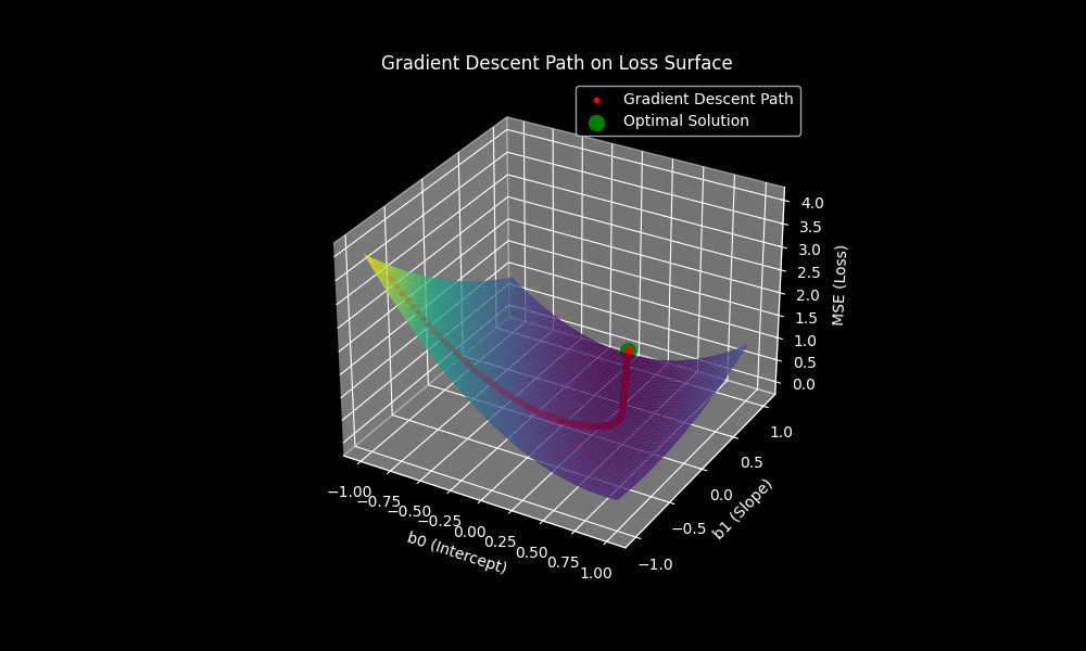
In most real-world scenarios, like fitting a line in linear regression ($y={\theta }_{1}x+{\theta }_0$), we need to optimize multiple parameters at once. The principle remains exactly the same. We just calculate the partial derivative for each parameter and update all of them simultaneously.

The set of all partial derivatives is the gradient, which is why the algorithm is called gradient descent.

Let's return to the StatQuest video to see how this works.

For a deeper dive into the specific math for deriving the gradients for Linear Regression's MSE cost function, you can review the following resource. Given your calculus background, you should be able to follow the application of the chain rule.

6. A Practical View: Gradient Descent in Code

Since you have an interest in coding, let's see how this all translates to Python. The video from NeuralNine, which we used before, also implements gradient descent from scratch. Watching this will solidify your understanding by connecting the mathematical theory to a working program.

7. A Note on A Practical Variation: Stochastic Gradient Descent (SGD)

In our examples, the gradient was calculated using all the data points. This is called Batch Gradient Descent. When you have millions of data points, this can be very slow.

A common and more efficient variant is Stochastic Gradient Descent (SGD), where the gradient is estimated using just one randomly selected data point at each step. A middle ground is Mini-Batch Gradient Descent, which uses a small random subset (a "mini-batch") of the data. This provides a good balance between accuracy and speed and is the most common method used in deep learning.

The StatQuest video provides a great, simple explanation of this.

Conclusion

Fantastic work today! You have just learned the single most important optimization algorithm in machine learning. This concept will reappear constantly as you study linear regression, logistic regression, and neural networks.

Key Takeaways:

• Gradient Descent is an iterative algorithm for finding the minimum of a function (the loss function).
• It works by repeatedly taking steps in the direction opposite to the gradient.
• The core update rule is ${\theta }_{\text{new}}={\theta }_{\text{old}}-\eta \nabla J({\theta }_{\text{old}})$.
• The learning rate ($\eta$) is a critical hyperparameter that controls the step size. If it's too large, the algorithm can diverge; if it's too small, it will be too slow.
• For functions with multiple parameters, we compute the gradient (vector of partial derivatives) and update all parameters simultaneously.
• Stochastic Gradient Descent (SGD) is a faster, more practical variant used for large datasets.

Preview of the Next Lesson:

Gradient descent is the go-to tool for the unconstrained optimization problems that dominate machine learning. However, sometimes we encounter problems where the variables must satisfy certain conditions or constraints. In our next lesson, we will explore a powerful analytical technique for these situations: the method of Lagrange multipliers. This will add another important optimization tool to your mathematical toolkit for the GATE exam.