Lagrange Multipliers for Constrained Optimization

1. The Challenge: Optimization with a Catch

Let's start with a visual. Imagine the surface below represents a function $f(x,y)$ we want to maximize or minimize (e.g., profit). The "level curves" on the left are like contours on a map, each one representing a constant value of the function.

Now, imagine we are not free to roam anywhere on this surface. We are restricted to a specific path, the "constraint" curve. Our goal is to find the highest and lowest points on the surface while staying on the path.

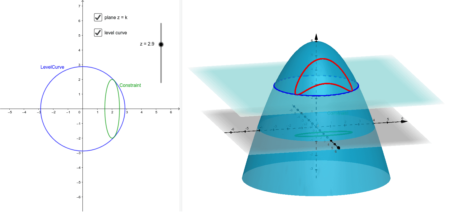
How can we find these optimal points?

2. The Geometric Insight: Tangency and Parallel Gradients

The key insight is geometric. As you move along the constraint path, the value of the function $f$ changes. The maximum (or minimum) value will occur at a point where the constraint curve just barely "kisses" or is tangent to one of the level curves of $f$.

Why? If the constraint curve crossed a level curve, it would mean you are moving from a region of lower function value to higher (or vice-versa). Therefore, the point of crossing can't be a maximum or a minimum. The extreme value must occur at the point of tangency.

Recall from our previous lessons on partial derivatives that the gradient vector ($\nabla f$) is always perpendicular (normal) to the level curve at any given point.

• If the constraint curve g = c and the level curve f = k are tangent at a point (x₀, y₀).
• And ∇g is normal to the constraint curve.
• And ∇f is normal to the level curve.
• Then at that point of tangency, the two gradient vectors ∇f and ∇g must be pointing in the same (or exactly opposite) directions. That is, they must be parallel.

Two vectors are parallel if one is a scalar multiple of the other. This gives us the central equation of the Lagrange multiplier method:

Here, $\lambda$ (the Greek letter lambda) is a scalar constant called the Lagrange multiplier.

This video provides an excellent visual and geometric explanation of this core idea.

3. The Method: A Step-by-Step Strategy

The geometric insight gives us a concrete method for solving constrained optimization problems. We simply need to find the point(s) (x, y) that satisfy both our constraint and the gradient condition.

For a problem where we want to optimize $f(x,y)$ subject to the constraint $g(x,y)=k$, we can use the following strategy.

To summarize and combine with our notation, the strategy is:

1. Identify Functions: Determine your objective function $f(x,y)$ to be maximized/minimized and your constraint function $g(x,y)=k$.
2. Calculate Gradients: Find the gradient of the objective function, $\nabla f=⟨\frac{\partial f}{\partial x},\frac{\partial f}{\partial y}⟩$, and the gradient of the constraint function, $\nabla g=⟨\frac{\partial g}{\partial x},\frac{\partial g}{\partial y}⟩$.
3. Set Up the System of Equations: Create a system of three equations with three unknowns ($x$, $y$, and $\lambda$):
   • $\frac{\partial f}{\partial x}=\lambda \frac{\partial g}{\partial x}$ (from the x-component of $\nabla f=\lambda \nabla g$)
   • $\frac{\partial f}{\partial y}=\lambda \frac{\partial g}{\partial y}$ (from the y-component of $\nabla f=\lambda \nabla g$)
   • $g(x,y)=k$ (the original constraint)
4. Solve the System: Solve the system of equations for $x$ and $y$. These are your candidate points for the maximum or minimum.
5. Evaluate: Plug the candidate point(s) back into the original function $f(x,y)$ to determine which gives the maximum and which gives the minimum value.

4. A Worked Example

Now, let's see this strategy in action. The same video we watched for the intuition also includes a complete, step-by-step algebraic solution to a problem.

5. Extension to More Variables and Constraints

The power of Lagrange multipliers is that the logic extends easily.

• Three Variables, One Constraint: To optimize $f(x,y,z)$ subject to $g(x,y,z)=k$, the system simply gets one more equation from the z-component of the gradient:

  $$\nabla f=\lambda \nabla g⟹\{\begin{array}{l}{f}_x=\lambda g_x\\ f_y=\lambda g_y\\ f_z=\lambda g_z\end{array}$$

  You would solve this along with the constraint $g(x,y,z)=k$.

• Two Constraints: Some problems, especially in engineering and physics, have multiple constraints. To optimize $f(x,y,z)$ subject to both $g(x,y,z)=k_1$ and $h(x,y,z)=k_2$, you introduce a second Lagrange multiplier, $\mu$. The gradient condition becomes:

  $$\nabla f=\lambda \nabla g+\mu \nabla h$$

  This will give you a system of 5 equations (3 from the gradient components, 2 from the constraints) with 5 unknowns ($x,y,z,\lambda ,\mu$). While more complex to solve, the principle is the same. The OpenStax resource LINK covers this case in the section "Problems with Two Constraints" if you'd like to see a full example.

6. Practical Application: Solving with Code

Since you have an interest in coding, it's great to see how this mathematical tool connects to programming. While solving complex systems of non-linear equations can be tricky, many problems result in a system of linear equations. We can use Python's NumPy library to solve these instantly, bypassing tedious manual algebra.

This is a very practical skill for an engineer. Let's see how it's done.

This approach powerfully combines your calculus knowledge with your coding skills to solve complex problems efficiently.

Conclusion

You've done an excellent job today! We have added a powerful new tool to your optimization toolkit. Where gradient descent helps us find optima in unconstrained spaces, Lagrange multipliers provide an elegant, analytical way to handle optimization with strict equality constraints.

Key Takeaways:

• Constrained optimization seeks to find the maximum or minimum of a function subject to certain conditions or constraints.
• The geometric intuition is that at an optimal point, the constraint curve is tangent to a level curve of the objective function.
• This tangency implies that the gradient vectors are parallel: $\nabla f=\lambda \nabla g$.
• This single vector equation, combined with the constraint equation, creates a system of equations that we can solve to find candidate points for the optima.
• The method extends to more variables and multiple constraints.
• For problems that result in a linear system, we can use tools like NumPy to find the solution computationally.

Preview of the Next Lesson:

We are now at the end of the "Calculus for Optimization" module. You have learned about derivatives, partial derivatives, finding optima, and methods for both unconstrained (gradient descent) and constrained (Lagrange multipliers) problems.

In our next lesson, we will change gears and begin the next major topic in calculus: integration. We will start with the Fundamental Theorem of Calculus, which establishes the profound link between differentiation and integration.