Optimizing Neural Networks with SGD and Adam

1. The Optimization Loop: Putting the Pieces Together

Training a neural network is an iterative process. In each iteration (or "step"), we perform three main actions:

1. Make a prediction and calculate the loss (the forward pass).
2. Calculate the gradients of the loss with respect to each parameter (the backward pass, using backpropagation).
3. Update the parameters using these gradients (the optimizer step).

This entire cycle is often called the training loop. An optimizer is the component responsible for step 3.

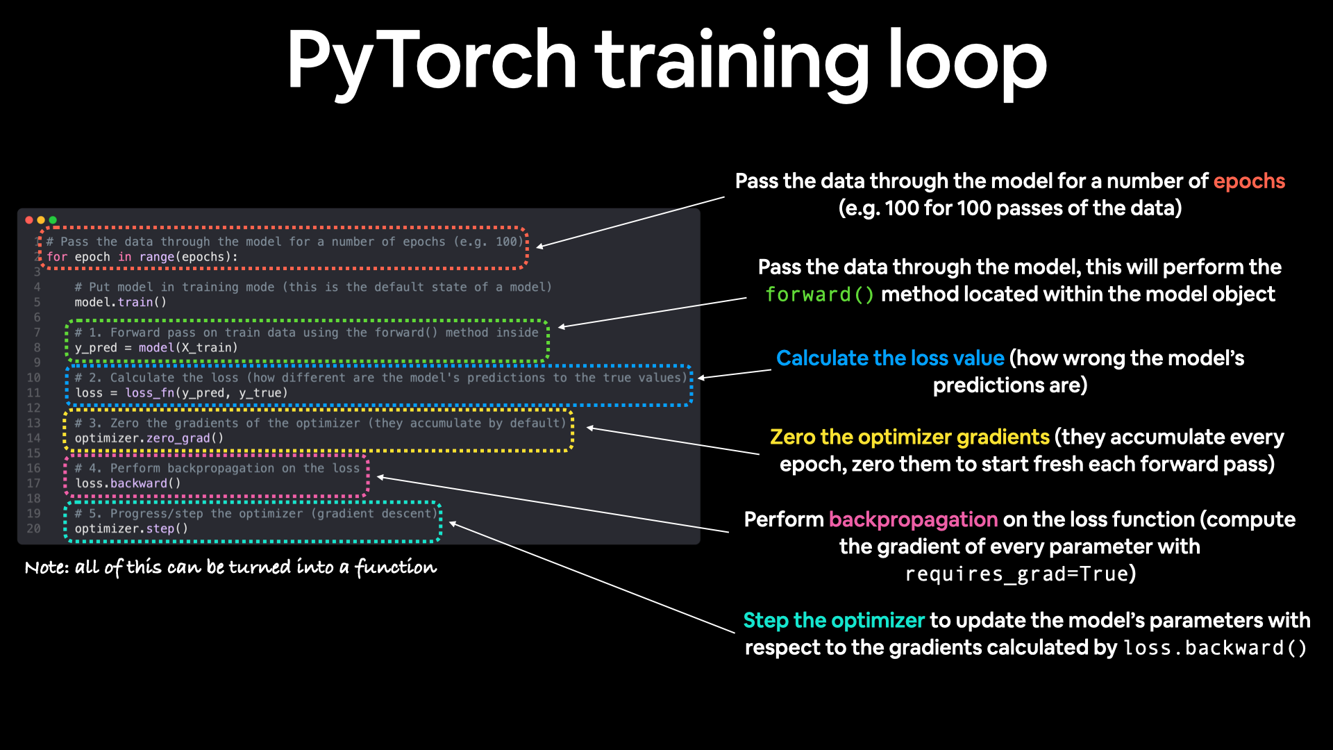
To control this process, we use hyperparameters. These are settings you, the developer, choose before training begins.

As the reading explains, the simplest optimization strategy is Gradient Descent. The update rule is straightforward:

The learning rate ($\alpha$) is a small positive number that controls the size of our update steps. The core of the training loop in PyTorch, which you will use repeatedly, looks like this:

# 1. Zero the gradients from the previous step
optimizer.zero_grad()

# 2. Perform the forward pass to get predictions
outputs = model(inputs)

# 3. Calculate the loss
loss = loss_fn(outputs, targets)

# 4. Perform the backward pass to calculate gradients
loss.backward()

# 5. Tell the optimizer to update the parameters
optimizer.step()

2. Stochastic Gradient Descent (SGD)

While "Gradient Descent" often refers to using the entire dataset to compute the gradient before taking one update step (also called Batch GD), this is computationally expensive.

In practice, we use Mini-Batch Stochastic Gradient Descent (SGD). Here, we calculate the gradient and update the parameters based on a small batch of data (e.g., 32 or 64 samples) instead of the whole dataset. This is much faster and provides a good-enough approximation of the true gradient. In deep learning, when people say "SGD", they almost always mean mini-batch SGD.

Let's see how PyTorch makes this easy.

To use SGD in PyTorch, you simply initialize it, telling it which parameters to optimize and what learning rate to use:

import torch.optim as optim

# model.parameters() tells the optimizer which tensors to update.
optimizer = optim.SGD(model.parameters(), lr=0.01) 

The rest of the training loop remains the same!

3. The Need for Better Optimizers

SGD is a great starting point, but it has some well-known issues:

• It can be very slow to converge if the loss landscape is shaped like a long, narrow ravine.
• It can get stuck in local minima or saddle points.
• The learning rate is the same for all parameters, which may not be ideal.

This has led to the development of more sophisticated optimizers that try to address these problems.

To build our intuition, let's explore these more advanced methods.

As the video explains, SGD with Momentum introduces a "velocity" term that accumulates an exponentially decaying average of past gradients. The intuition is like a ball rolling down a hill: it builds up momentum and can power through small bumps (local minima) and move faster in consistent directions.

The update looks like this:

Here, $v_t$ is the velocity at time $t$, and $\beta$ is the momentum coefficient (often set to 0.9).

4. Adaptive Learning Rates: RMSprop and Adam

Another major improvement was the idea of adaptive learning rates, where each parameter gets its own learning rate that changes during training.

RMSprop (Root Mean Square Propagation) is one such algorithm. It divides the learning rate for a weight by a running average of the magnitudes of recent gradients for that weight. This means:

• Parameters with large gradients get smaller updates.
• Parameters with small gradients get larger updates.

This helps tremendously in ravine-shaped loss landscapes, dampening the oscillations in the steep direction and accelerating progress in the flatter direction.

Now, let's see what happens when we combine these two powerful ideas.

Adam has become the de-facto standard optimizer for most deep learning applications. It combines:

1. Momentum: It keeps an exponentially decaying average of past gradients (the "first moment").
2. Adaptive Learning Rates: It also keeps an exponentially decaying average of past squared gradients, similar to RMSprop (the "second moment").

It is generally robust, effective, and requires less manual tuning of the learning rate compared to SGD.

In PyTorch, using Adam is just as simple as using SGD:

# A common learning rate for Adam is 0.001
optimizer = optim.Adam(model.parameters(), lr=0.001)

5. Practical Considerations

While you won't need to implement these optimizers from scratch for the GATE exam (as you'll use libraries like PyTorch), understanding their behavior is key.

As a final recap, let's look at the benchmarks presented in the video "Who's Adam and What's He Optimizing?".

The general consensus is: start with Adam. It is a fantastic default. If you run into issues or need to squeeze out the last bit of performance for a specific task, you might then experiment with SGD with Momentum or other advanced optimizers.

Conclusion

Congratulations! You now understand the final piece of the training puzzle. We've gone from a forward pass, to a backward pass, and now to the optimizer step that puts it all into action.

Key Takeaways:

• Optimizers use the gradients from backpropagation to update the model's parameters and minimize the loss.
• The training loop consists of a forward pass, a backward pass, and an optimizer step, repeated over many epochs.
• Stochastic Gradient Descent (SGD) is the foundational optimizer, but it can be slow and unstable.
• Momentum helps accelerate SGD by adding a "velocity" term, smoothing updates and overcoming small local minima.
• Adam is a powerful adaptive optimizer that combines the ideas of momentum and per-parameter adaptive learning rates (like RMSprop). It is the recommended default choice for most deep learning tasks.
• In PyTorch, using any optimizer follows the same pattern: initialize it, then call optimizer.zero_grad(), loss.backward(), and optimizer.step() inside your training loop.

Preview of the Next Lesson:
We have now covered all the individual components required to train a neural network. In the next lesson, "Implement a complete training loop in PyTorch," we will put everything together—data loading, model definition, forward pass, loss calculation, backward pass, and optimizer updates—to write a complete Python script that trains a neural network from start to finish on a real dataset.