Backpropagation: Computing Gradients

Hello! Welcome back to our journey into Deep Learning with PyTorch.

In the last lesson, we successfully implemented the forward pass. We saw how input data travels through the layers of a neural network to produce a prediction, and how we can use a loss function, like nn.CrossEntropyLoss, to calculate a single number representing the network's error.

But a single error number is just a score. How does the network actually learn from it? The goal of this lesson is to answer that question by explaining the backpropagation algorithm for computing gradients. We will demystify the core mechanism that enables a neural network to adjust its internal parameters (weights and biases) to improve its performance.

By the end of this 60-minute lesson, you will be able to:

Intuitively explain how an error signal is propagated backward through a network.
Understand the role of the chain rule in calculating gradients.
Describe how the sensitivity of the loss to each weight and bias is computed.

Let's begin!

1. From Error to "Desired Nudges": The Intuition of Backpropagation

The forward pass is a journey from input to error. Backpropagation is the return journey, where the network figures out how to correct its mistakes. The "mistake" is quantified by the loss function. The "correction" involves slightly nudging every single weight and bias in the network in a direction that will reduce that loss.

The central question is: how much should we nudge each parameter? And in which direction (increase or decrease)?

Backpropagation is the algorithm that answers this. It calculates the gradient of the loss function with respect to every parameter in the network. Think of the gradient as a measure of "sensitivity": it tells us how sensitive the final loss is to a tiny change in each weight and bias. A large gradient for a specific weight means changing that weight will have a big impact on the loss.

Let's start by building a strong intuition for this process.

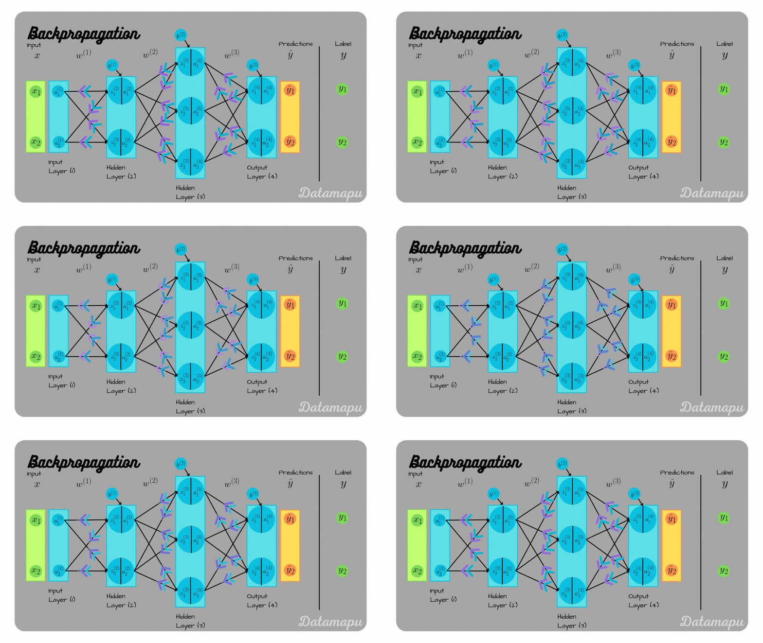
Animated Illustration of Backpropagation in a Neural Network — This animation shows the two phases of training. First, the **forward pass** (left to right) computes the prediction and loss. Then, the **backward pass** (right to left) propagates the error signal back through the network to calculate the gradients needed for updates.

The following video from 3Blue1Brown is one of the best explanations available for the intuition behind backpropagation. It masterfully explains the concepts without getting bogged down in complex formulas.

Backpropagation, intuitively | Deep Learning Chapter 3

Let's watch 'Backpropagation, intuitively' by 3Blue1Brown. This video will help you understand what backpropagation is actually doing conceptually.

Please watch from the beginning until 08:28. As you watch, focus on these key ideas: How the desired change in the output layer (e.g., wanting the '2' neuron to be more active and others less) creates a set of 'nudges'. How the influence of a weight is related to the activation of the neuron it's connected to. How the desired changes from the output layer are propagated backward to determine the desired changes for the previous layers.

To summarize the core ideas from the video:

The process starts at the end. We know what the output should have been. The difference between the actual output and the desired output tells us how to adjust the activations in the final layer.
To change an activation, we can change the weights and biases connected to it. The most effective weights to change are those connected to the brightest (most active) neurons in the previous layer. This is a key insight often summarized as "neurons that fire together, wire together."
This desire for change is then propagated backward. The neurons in the second-to-last layer receive a combined "wish list" of changes from all the neurons in the output layer they are connected to.
This process repeats, layer by layer, all the way back to the start of the network. At the end, we have a "desired nudge" for every single weight and bias. This collection of nudges is the gradient.

2. Making it Concrete: Computational Graphs

The intuitive idea of "propagating desires" is powerful, but to implement it, we need a more formal structure. A computational graph is a perfect tool for this. It visualizes the entire sequence of operations in the forward pass as a directed graph.

Every mathematical operation (addition, multiplication, activation function) is a node, and the arrows show how the output of one node becomes the input for another. Backpropagation simply involves moving backward along these arrows, calculating the local gradient at each node, and passing it on.

Computational Graphs, Forward Propagation, and ...

This article, 'Computational Graphs, Forward Propagation, and Backward Propagation for Nueral Networks,' provides a clear, step-by-step walkthrough of backpropagation using a simple computational graph. This will help formalize the intuition we just built.

Please read the introduction and the first main section about the simple computational graph example (until the first block of Python code). Focus on understanding the following terms: Forward Pass: Calculating the final output. Backward Pass: Moving backward from the output to calculate gradients. Upstream Gradient: The gradient coming from a node's successor in the graph. Local Gradient: The gradient of a node's output with respect to its immediate input. Chain Rule: How the upstream and local gradients are combined (downstream_gradient = upstream_gradient * local_gradient).

The key takeaway is the application of the chain rule from calculus. If a variable x affects q, and q affects F, the chain rule tells us how to find the effect of x on F:

$\frac{\partial F}{\partial x} = \frac{\partial F}{\partial q} \cdot \frac{\partial q}{\partial x}$

In our graph terminology:

$\frac{\partial F}{\partial q}$ is the upstream gradient.
$\frac{\partial q}{\partial x}$ is the local gradient.
$\frac{\partial F}{\partial x}$ is the downstream gradient we want to compute.

Backpropagation is just a recursive application of this rule, moving from the final loss all the way back to the first-layer weights.

3. The Calculus of Backpropagation

Now that we have both the intuition and a visual model, let's look at the underlying mathematics. We'll use the same notation and simple network structure from 3Blue1Brown's calculus explanation. Don't worry about memorizing these formulas; the goal is to see how the chain rule directly translates into the update steps.

Let's use the excellent text-based explanation that accompanies the video, as it allows you to go through the math at your own pace.

Backpropagation calculus - 3Blue1Brown

The article 'Backpropagation calculus' from 3Blue1Brown provides the mathematical formulas that formalize the process. We will walk through the simplest case to understand the core mechanics.

Read the sections 'Calculating the Gradient with Backpropagation', 'Computing The First Derivative', and 'The Constituent Derivatives' (up to 'Putting It All Together'). Pay attention to how the derivative of the cost with respect to a weight, \frac{\partial C_0}{\partial w^{(L)}}, is broken down into three simpler derivatives using the chain rule.

Let's break down the central formula from the reading. For the last layer $L$ , the sensitivity of the cost $C_{0}$ with respect to a single weight $w^{(L)}$ is:

\frac{\partial C _{0}}{\partial w ^{(L)}} = \frac{\partial z ^{(L)}}{\partial w ^{(L)}} \cdot \frac{\partial a ^{(L)}}{\partial z ^{(L)}} \cdot \frac{\partial C _{0}}{\partial a ^{(L)}}

Let's connect this back to our intuition:

$\frac{\partial C _{0}}{\partial a ^{(L)}} = 2 (a^{(L)} - y)$
- This is the error in the output. How far was the final activation $a^{(L)}$ from the desired value $y$ ? The bigger the error, the more we need to change things.
$\frac{\partial a ^{(L)}}{\partial z ^{(L)}} = σ^{'} (z^{(L)})$
- This is the derivative of the activation function. It tells us how much the activation $a^{(L)}$ will change for a small nudge in its input $z^{(L)}$ .
$\frac{\partial z ^{(L)}}{\partial w ^{(L)}} = a^{(L - 1)}$
- This is the activation of the previous layer's neuron. A nudge to the weight $w^{(L)}$ has a larger effect on $z^{(L)}$ if the neuron connected to it, with activation $a^{(L - 1)}$ , is firing strongly. This is the mathematical form of "neurons that fire together, wire together."

Multiplying these three terms together gives us the gradient for one weight. Backpropagation is simply the algorithm that computes these products efficiently for all weights and biases, moving backward layer by layer.

Test your understanding!

Consider the term $\frac{\partial z ^{(L)}}{\partial w ^{(L)}} = a^{(L - 1)}$ . If the activation of a neuron in the previous layer, $a^{(L - 1)}$ , is close to zero, what does this imply about the gradient of the weight $w^{(L)}$ connecting it to the next layer? How does this relate to the "fire together, wire together" idea?

Show answer

If $a^{(L - 1)}$ is close to zero, the gradient $\frac{\partial C _{0}}{\partial w ^{(L)}}$ will also be close to zero, because $a^{(L - 1)}$ is one of the terms being multiplied. This means that the weight will be updated very little, if at all.

This directly relates to "fire together, wire together." If the neuron in the previous layer isn't firing ( $a^{(L - 1)} \approx 0$ ), it doesn't matter how much error there is in the next layer; the connection (weight) is not considered responsible and therefore isn't changed much. The network only strongly updates connections between neurons that are both active.

In practice, libraries like PyTorch handle all of this for you when you call loss.backward(). But understanding what happens under the hood is crucial for debugging, designing better models, and truly grasping how deep learning works.

Conclusion

Today, we've pulled back the curtain on the "magic" of how neural networks learn.

Key Takeaways:

Backpropagation is an efficient algorithm that computes the gradient of the loss function with respect to every weight and bias in the network.
It works by applying the chain rule from calculus, starting from the final layer and moving backward through the network's computational graph.
The calculated gradient for a parameter tells us how sensitive the loss is to changes in that parameter. This gives us the direction and relative magnitude of the "nudge" needed to improve the network.
The process can be understood intuitively ("neurons that fire together, wire together"), visually (computational graphs), and mathematically (the chain rule).

Preview of the Next Lesson:
We now have a forward pass to make predictions and a backward pass (backpropagation) to find the gradients. We're missing the final piece: actually using those gradients to update the network's parameters. In the next lesson, "Train a neural network using stochastic gradient descent (SGD) and its variants like Adam," we will learn about the optimization algorithms that perform these updates and bring the entire training loop together.

Recommended resources

1. From Error to "Desired Nudges": The Intuition of Backpropagation

2. Making it Concrete: Computational Graphs

3. The Calculus of Backpropagation

Conclusion