Implementing the Full Forward Pass

1. The Journey of Data: Understanding the Forward Pass

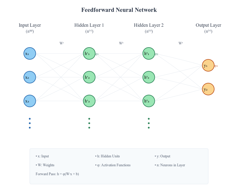
The forward pass is the process a neural network uses to turn an input into an output. It's a sequence of simple steps, repeated layer by layer. The output of one layer becomes the input for the next.

Let's break down the core concepts before jumping into code.

As you just read, the process for each layer can be summarized in two steps:

1. Linear Transformation: Calculate a weighted sum of the inputs and add a bias. If your input is A_prev (activations from the previous layer), the calculation is:
   $Z=W\cdot A_{prev}+b$
   This uses the matrix multiplication skills you learned in the Linear Algebra module. W is the weight matrix for the current layer and b is its bias vector. Z is often called the "pre-activation" or "logit".

2. Activation: Pass the result Z through a non-linear activation function. This is where your knowledge from the last lesson comes in.
   $A=\text{activation}(Z)$
   The result A is the output of the current layer, which then serves as the input A_prev for the next layer.

This entire chain of operations, from the initial input X to the final output, is the forward pass.

2. Building a Neural Network in PyTorch

Now, let's translate this concept into code. In PyTorch, we define our network's architecture by creating a class that inherits from torch.nn.Module. This class has two essential methods:

• __init__(): This is the constructor. Here, you define all the layers your network will use, like linear layers (nn.Linear) and activation functions (nn.ReLU). These layers are stored as attributes of the class.
• forward(): This method defines the data flow. You take an input tensor x and explicitly pass it through the layers you defined in __init__, in the correct sequence.

Let's watch a practical demonstration of how to set this up for a simple feedforward network.

As you saw in the video, the forward method is where the magic happens. It's a direct implementation of the process we discussed: a linear layer, followed by an activation, followed by the next linear layer.

Notice a very important detail: we don't apply the Softmax activation function in the forward method. This is a common practice in PyTorch because the recommended loss function for classification, nn.CrossEntropyLoss, combines both the Softmax activation and the loss calculation in one efficient step. We'll get to that next.

3. Computing Predictions and Loss

Once the network is defined, performing the forward pass is as simple as calling the model instance with your input data.

# Assuming 'model' is an instance of our NeuralNet class
# and 'images' is a batch of input data
outputs = model(images) 

This single line executes the entire forward method and gives you the final raw scores (logits) from the network.

But how do we know if these outputs are good? We need to compare them to the ground truth (the correct labels) and quantify the error. This is the job of a loss function (or criterion).

For a multi-class classification problem like recognizing digits, the standard loss function is Cross-Entropy Loss.

• What it does: It measures the performance of a classification model whose output is a probability value between 0 and 1. Cross-entropy loss increases as the predicted probability diverges from the actual label.
• In PyTorch: We use nn.CrossEntropyLoss. As mentioned, this function expects the raw, unnormalized scores (logits) directly from your model's final linear layer. It applies the Softmax function internally before calculating the loss.

Let's see this final step in action.

4. A Complete Example

Let's put all the pieces together in a single, runnable code block. Here, we will:

1. Import PyTorch.
2. Define a simple NeuralNetwork class.
3. Instantiate the model and the loss function.
4. Create a dummy batch of input data and corresponding labels.
5. Perform a full forward pass to get predictions and calculate the loss.

import torch
import torch.nn as nn

# 1. Define the network architecture
class NeuralNetwork(nn.Module):
    def __init__(self, input_size, hidden_size, num_classes):
        super(NeuralNetwork, self).__init__()
        self.layer1 = nn.Linear(input_size, hidden_size) 
        self.relu = nn.ReLU()
        self.layer2 = nn.Linear(hidden_size, num_classes)  
    
    def forward(self, x):
        # Pass data through the first linear layer
        out = self.layer1(x)
        # Apply ReLU activation
        out = self.relu(out)
        # Pass through the final linear layer to get logits
        out = self.layer2(out)
        return out

# 2. Set Hyperparameters and Instantiate Model
input_size = 784  # e.g., 28x28 flattened images
hidden_size = 100
num_classes = 10  # e.g., digits 0-9
batch_size = 5

model = NeuralNetwork(input_size, hidden_size, num_classes)

# 3. Define the Loss Function
criterion = nn.CrossEntropyLoss()

# 4. Create Dummy Data
# A batch of 5 "images", each flattened to 784 features
dummy_input = torch.randn(batch_size, input_size) 
# True labels for the 5 images (e.g., image 0 is class 3, image 1 is class 0, etc.)
dummy_labels = torch.tensor([3, 0, 8, 5, 9]) 

print(f"Shape of input data: {dummy_input.shape}")
print(f"Shape of labels: {dummy_labels.shape}")

# 5. Perform the Forward Pass and Calculate Loss
# Get model predictions (logits)
outputs = model(dummy_input)
print(f"\nShape of model outputs (logits): {outputs.shape}")

# Calculate the loss
loss = criterion(outputs, dummy_labels)
print(f"Calculated Loss: {loss.item()}") 

This script encapsulates everything we've learned today. It defines the path data takes (forward), pushes the data through that path (model(dummy_input)), and then computes the error (criterion(outputs, dummy_labels)).

Conclusion

Congratulations! You have successfully implemented the core prediction mechanism of a neural network. This forward pass is the foundation upon which all training is built.

Key Takeaways:

• The forward pass is the sequence of operations that takes an input and produces a prediction.
• In PyTorch, we define a network's structure by creating a class that inherits from nn.Module.
• The __init__ method is used to define the layers of the network (e.g., nn.Linear).
• The forward method is used to define the data's path through those layers.
• A loss function (like nn.CrossEntropyLoss) quantifies the error by comparing the model's output (logits) to the true labels.

Preview of the Next Lesson:
We now know how to get a prediction and measure its error. But how do we use that error to make the network better? That's the job of backpropagation. In the next lesson, "Explain the backpropagation algorithm for computing gradients," we will explore the mechanism that allows the network to learn from its mistakes by adjusting its weights and biases.