NumPy Array and Matrix Operations

1. What is NumPy and Why is it Essential?

NumPy (short for Numerical Python) is a library that provides a powerful object called an N-dimensional array (or ndarray). Think of it as a highly efficient, supercharged version of a Python list that is optimized for mathematical operations.

Why not just use Python lists?

• Speed: NumPy operations are written in C, a low-level language, which makes them much faster than equivalent operations on Python lists.
• Memory Efficiency: NumPy arrays store data more compactly.
• Convenience: NumPy provides a huge number of built-in functions for linear algebra, statistical analysis, and other mathematical tasks.

As you learned in the previous lesson, we need to import a library to use it. The standard convention, which you will see everywhere in the data science world, is to import NumPy with the alias np.

import numpy as np

From now on, we will use np to access all of NumPy's functions.

2. Creating NumPy Arrays

The most fundamental step is creating a NumPy array. You can create one from a standard Python list.

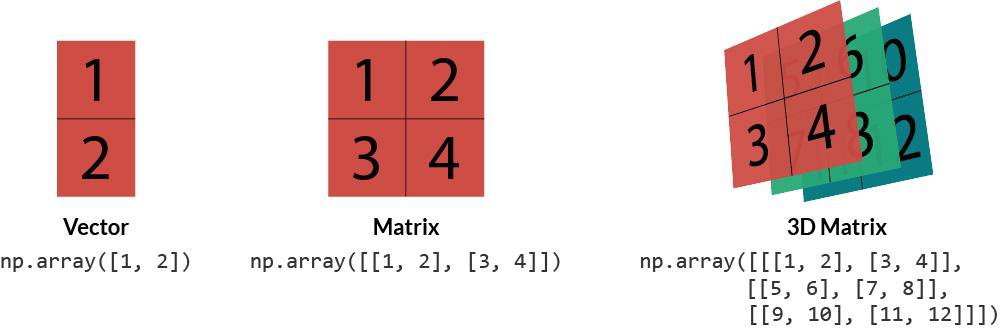
• A 1D array (or a vector) is created from a simple list.
• A 2D array (or a matrix) is created from a list of lists.

# Create a 1D array (vector)
vec = np.array([1, 2, 3, 4])
print("Vector:")
print(vec)

# Create a 2D array (matrix)
mat = np.array([[1, 2, 3], [4, 5, 6]])
print("\nMatrix:")
print(mat)

The image below illustrates these fundamental structures.

Let's watch a short video segment that demonstrates the basic initialization of these arrays.

Besides creating arrays from lists, NumPy provides handy functions to create arrays with initial placeholder content. This is very useful when you know the size of the array you need but not the values yet.

• np.zeros((rows, cols)): Creates an array of a given shape filled with zeros.
• np.ones((rows, cols)): Creates an array filled with ones.
• np.arange(start, stop, step): Creates an array with a range of numbers, similar to Python's range().

# A 3x4 matrix of zeros
zeros_matrix = np.zeros((3, 4))
print(zeros_matrix)

# A 1D array of five ones
ones_vector = np.ones(5)
print("\n", ones_vector)

# An array of even numbers from 2 up to (but not including) 10
evens = np.arange(2, 10, 2)
print("\n", evens)

3. Inspecting Your Arrays: Shape, Size, and Type

Once you have an array, you'll often need to know its properties. NumPy arrays have several useful attributes:

• .shape: A tuple representing the dimensions of the array (e.g., (2, 3) for a 2x3 matrix).
• .ndim: The number of dimensions (e.g., 1 for a vector, 2 for a matrix).
• .size: The total number of elements in the array.
• .dtype: The data type of the elements (e.g., int64, float64).

The following video segment will walk you through these attributes.

4. Accessing Elements: Indexing and Slicing

Just like with Python lists, you often need to select specific elements or sections of an array. NumPy uses a similar square bracket [] notation, but with some powerful extensions for multiple dimensions.

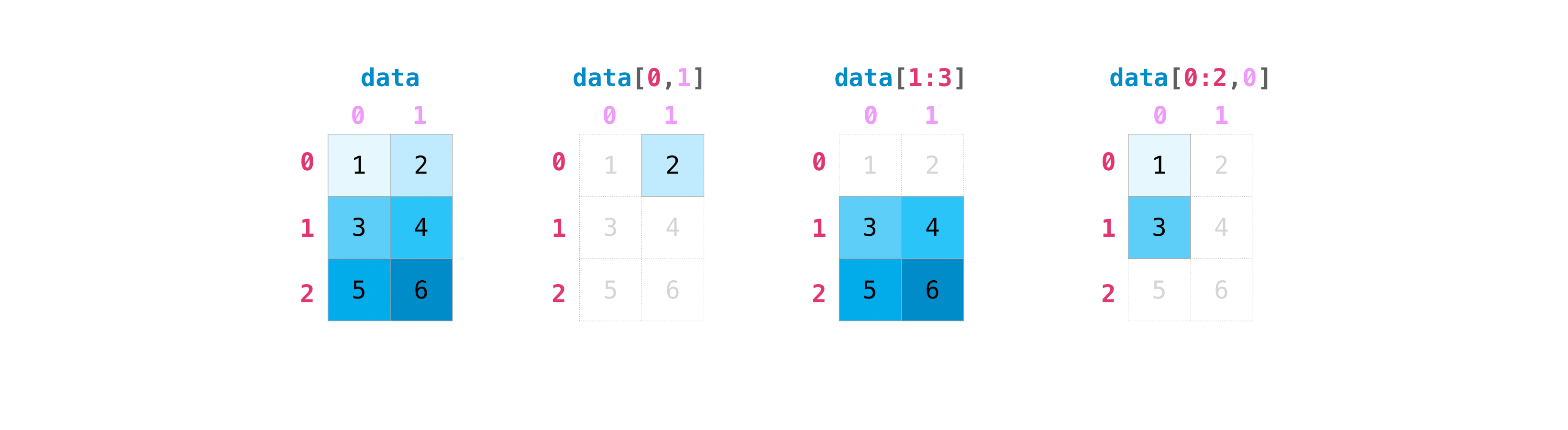
For a 2D array (matrix), you use the syntax array[row, column].

• A single number selects that row/column: mat[0, 1] selects the element in the first row, second column.
• A colon : selects all rows/columns: mat[:, 1] selects all rows from the second column.
• A range start:stop selects a slice: mat[0:2, :] selects the first two rows.

Watching this in action makes it much clearer.

import numpy as np
A = np.array([[10, 20, 30, 40],
              [50, 60, 70, 80],
              [90, 100, 110, 120]])

5. Array and Matrix Operations

This is where NumPy truly shines.

Element-wise Operations

Standard arithmetic operators (+, -, *, /) apply the operation element-by-element. If you add two arrays of the same shape, the corresponding elements are added together.

A = np.array([[1, 2], [3, 4]])
B = np.array([[10, 20], [30, 40]])

# Element-wise addition
print(A + B)
# [[11 22]
#  [33 44]]

# Element-wise multiplication
print(A * B)
# [[ 10  40]
#  [ 90 160]]

You can also perform operations with a single number (a scalar), and NumPy will apply it to every element. This is a concept called broadcasting.

# Add 100 to every element
print(A + 100)
# [[101 102]
#  [103 104]]

Matrix Multiplication

This is a crucial concept, especially for your future studies in linear algebra and machine learning. In mathematics, matrix multiplication is different from element-wise multiplication.

In NumPy, the * operator is for element-wise multiplication, NOT matrix multiplication.

To perform true matrix multiplication, you should use the @ operator (or the np.matmul() function).

For two matrices to be multiplied, the number of columns in the first matrix must equal the number of rows in the second.

• A (2, 3) matrix can be multiplied by a (3, 4) matrix. The result will be a (2, 4) matrix.
• A (2, 3) matrix cannot be multiplied by a (2, 3) matrix.

A = np.array([[1, 2, 3], [4, 5, 6]])  # Shape: (2, 3)
B = np.array([[7, 8], [9, 10], [11, 12]]) # Shape: (3, 2)

# Matrix multiplication
C = A @ B
print(C)
# [[ 58  64]
#  [139 154]]

print("Shape of A:", A.shape)
print("Shape of B:", B.shape)
print("Shape of C:", C.shape)

The following video demonstrates both element-wise math and matrix multiplication.

For an additional, very clear text explanation of this important difference, please review the following resource.

6. Aggregations and Other Manipulations

NumPy makes it easy to perform aggregations on arrays, like finding the sum, mean, or maximum value.

A = np.array([[1, 2, 3], [4, 5, 6]])

print(A.sum())    # Sum of all elements
print(A.mean())   # Mean of all elements
print(A.min())    # Minimum element
print(A.max())    # Maximum element

A powerful feature is the ability to perform these aggregations along a specific axis.

• axis=0 collapses the rows and performs the operation down each column.
• axis=1 collapses the columns and performs the operation across each row.

# Sum down the columns (axis=0)
print(A.sum(axis=0))  # [1+4, 2+5, 3+6] -> [5, 7, 9]

# Sum across the rows (axis=1)
print(A.sum(axis=1))    # [1+2+3, 4+5+6] -> [6, 15]

Two other common manipulations are:

• Reshaping: Changing the shape of an array with .reshape(). The new shape must have the same total number of elements.
• Transposing: Flipping a matrix over its diagonal with .T. This swaps the rows and columns.

A = np.arange(6) # [0, 1, 2, 3, 4, 5]

# Reshape into a 2x3 matrix
B = A.reshape(2, 3)
print(B)
# [[0 1 2]
#  [3 4 5]]

# Transpose the matrix
print(B.T)
# [[0 3]
#  [1 4]
#  [2 5]]

Conclusion

Excellent work! You've just learned the fundamentals of NumPy, the library that powers a huge portion of the data science ecosystem in Python. These skills are not just foundational; they are practical tools you will use constantly.

Key Takeaways:

• NumPy's ndarray is a fast and efficient data structure for numerical data.
• Arrays are created using np.array(), np.zeros(), np.arange(), and other functions.
• You can access array elements and sections using indexing [row, col] and slicing start:stop.
• Arithmetic operators (+, *) perform element-wise operations.
• The @ operator performs true matrix multiplication.
• Aggregation functions (.sum(), .mean()) can be applied to the whole array or along a specific axis.
• You can change an array's structure with .reshape() and .T.

In our next and final lesson for this module, we will learn how to load, manipulate, and analyze data using the Pandas library. You will see that the NumPy arrays and operations you've mastered today are the engine running under the hood of Pandas DataFrames, making this lesson the perfect preparation for working with real-world datasets.