Pandas Data Structures: Series & DataFrames

1. The Core Components of Pandas: Series and DataFrame

Pandas introduces two primary data structures that you'll use constantly: the Series and the DataFrame.

• A Series is a one-dimensional labeled array, much like a NumPy array but with an explicit index. You can think of it as a single column of data.
• A DataFrame is a two-dimensional labeled data structure, like a table in a spreadsheet or a SQL database. It has both a row index and column names.

The easiest way to think about their relationship is that a DataFrame is a collection of Series objects that share the same index.

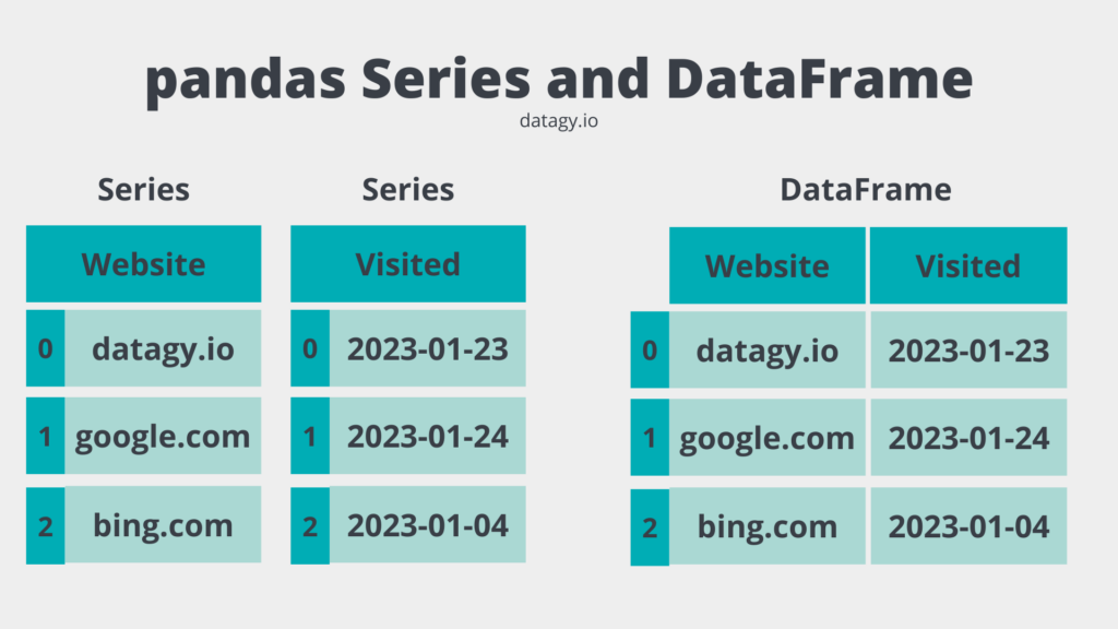
A DataFrame has a clear structure with an index for rows and names for columns.

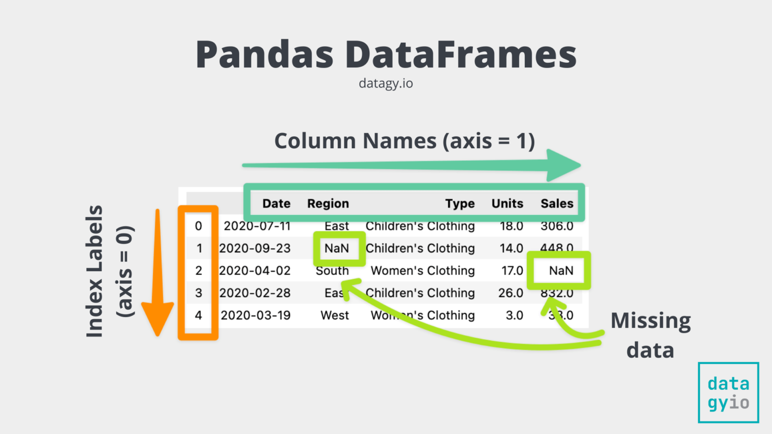
To see how these structures are created and how they relate to the Python dictionaries you already know, let's watch a short video.

As is standard practice, we'll import Pandas with the alias pd.

import pandas as pd

2. Loading Data into a DataFrame

While creating DataFrames from dictionaries is useful, in most data science tasks, you will load data from an external file. The most common format is a CSV (Comma-Separated Values) file.

Pandas makes this incredibly easy with the pd.read_csv() function. You simply provide the path to the file, and Pandas will parse it into a DataFrame.

Let's see how this works in practice. The following video will show you how to load a sample CSV file.

3. Inspecting and Understanding Your Data

Once you've loaded your data, the first step is always to inspect it to understand its structure and content. Pandas provides several essential methods for this initial exploration.

Let's assume we've loaded our data into a DataFrame called df (a common convention).

• df.head(): Shows the first 5 rows. You can pass a number like df.head(10) to see more.
• df.tail(): Shows the last 5 rows.
• df.shape: Returns a tuple (rows, columns), just like in NumPy.
• df.info(): Provides a concise summary, including the number of entries, the data type of each column, and the number of non-null values. This is extremely useful for spotting missing data.
• df.describe(): Generates descriptive statistics (count, mean, standard deviation, min, max, etc.) for all numerical columns.

The next video segment demonstrates these essential inspection methods.

4. Manipulating Data: Selection and Filtering

This is where you'll spend a lot of your time as a data analyst—pulling out the specific pieces of data you need.

Selecting Columns

• To select a single column, use square brackets [] with the column's name. This returns a Pandas Series.

  # Select the 'Product' column
  products = df['Product'] 
  

• To select multiple columns, use double square brackets [[]] with a list of column names. This returns a new DataFrame.

  # Select the 'Product' and 'Price' columns
  product_details = df[['Product', 'Price']]
  

Selecting Rows and Columns with .loc and .iloc

Pandas provides two powerful indexers for more advanced selection:

• .loc: Selects data by label. You use the index labels for rows and column names for columns.
• .iloc: Selects data by integer position. You use integer indices for both rows and columns, just like in NumPy.

# Select the row with index label 3
df.loc[3]

# Select the row at integer position 3 (the 4th row)
df.iloc[3]

# Select rows with labels 3 through 5, and columns 'Product' to 'Price'
df.loc[3:5, 'Product':'Price']

# Select rows at positions 3 through 5, and columns at positions 2 through 4
df.iloc[3:6, 2:5] # Note: iloc is exclusive of the end position for slicing, like Python lists

Conditional Filtering

This is one of the most powerful features of Pandas. You can filter your DataFrame based on conditions, similar to a WHERE clause in SQL.

# Get all orders from the 'USA'
usa_orders = df[df['Country'] == 'USA']

# Get all orders where the quantity is greater than 2
high_quantity_orders = df[df['Quantity'] > 2]

# You can combine conditions using `&` (and) and `|` (or).
# IMPORTANT: Each condition must be wrapped in parentheses.
electronics_in_usa = df[(df['Category'] == 'Electronics') & (df['Country'] == 'USA')]

The following videos will give you a practical demonstration of these selection and filtering techniques.

sales_df.loc[(sales_df['Country'] == 'India') & (sales_df['Price'] > 500), ['Product', 'Price']]

5. Basic Data Analysis and Aggregation

Once you can select and filter data, you can start analyzing it.

Value Counts

For categorical data, value_counts() is a quick way to see the distribution of items.

# Count the number of orders per country
df['Country'].value_counts()

GroupBy

The groupby() method is used for "split-apply-combine" operations. This is a powerful pattern in data analysis:

1. Split the data into groups based on some criteria.
2. Apply a function to each group independently.
3. Combine the results into a data structure.

For example, to find the average price of products in each category:

# Group by category, then find the mean of the 'Price' column for each group
df.groupby('Category')['Price'].mean()

This next video segment demonstrates these powerful, one-line analysis methods.

Conclusion

Congratulations on completing the first module! You have built a solid foundation in Python, from basic syntax to the powerful data manipulation capabilities of NumPy and now Pandas. These are the tools you will rely on throughout your data science journey.

Key Takeaways:

• Pandas provides two main data structures: the 1D Series and the 2D DataFrame.
• Data is most commonly loaded from files using functions like pd.read_csv().
• You should always start by inspecting your data with .head(), .info(), and .describe().
• You can manipulate data by selecting columns with [], and selecting specific rows and columns with .loc (label-based) and .iloc (position-based).
• Conditional filtering (df[df['column'] > value]) is essential for isolating data that meets specific criteria.
• You can begin to analyze data using .value_counts() for distributions and .groupby() for calculating statistics on subsets of your data.

This lesson marks the end of our "Python for Data Science: Foundations" module. You've acquired the essential programming skills needed to handle data. In the next module, "Mathematical Foundations: Linear Algebra," we will shift gears. You will learn the mathematical principles that power many of the advanced algorithms used in data science and machine learning. Your ability to work with data in NumPy and Pandas will be the perfect practical counterpart to the theoretical concepts you're about to explore.