Hello! Welcome to the start of a new and exciting module: Graph Algorithms.
In our last lesson, we concluded our study of specialized data structures by contrasting Segment Trees and Fenwick Trees. We learned that the choice between them hinges on deep trade-offs between flexibility, memory, and the mathematical properties of the required operation.
Today, we bring that same analytical mindset to a new domain. Graphs are one of the most versatile data structures in computer science, modeling everything from social networks to distributed systems. Before we can solve problems on them, we must first understand how to store them. Your learning outcome for this lesson is to represent graphs using adjacency lists and matrices, and analyze their space-time trade-offs. Mastering this foundational topic is the critical first step toward tackling the complex graph problems favored in elite technical interviews.
1. The Five Concepts for Today
We will break down today's topic into five interrelated concepts, moving from foundational definitions to deep trade-off analysis:
- What is a Graph? The basic vocabulary of nodes, edges, and their properties.
- Adjacency Matrix: Representing connections in a grid.
- Adjacency List: Representing connections as lists of neighbors.
- Space Complexity Trade-offs: The "Sparse vs. Dense" dilemma.
- Time Complexity Trade-offs: Analyzing the performance of key operations.
Concept 1: What is a Graph?
Technical Explanation
A graph is a data structure used to represent relationships or connections between objects. It's formally defined as a pair of sets, , where:
- is a set of vertices (or nodes), which represent the objects.
- is a set of edges, which represent the connections between pairs of vertices.
Graphs can have several properties:
- Directed vs. Undirected: An undirected edge
(u, v)implies a two-way relationship (like a friendship on Facebook). A directed edge(u, v)implies a one-way relationship (like following someone on Twitter). - Weighted vs. Unweighted: A weighted edge has a "cost" or "distance" associated with it (like the distance between two cities on a map). In an unweighted graph, all edges are considered equal.
- Cyclic vs. Acyclic: A cycle is a path that starts and ends at the same vertex.
For a great overview of this terminology and its relevance, the following resource is very helpful.
Graph Interview Questions & Tips for Senior Engineers
The article 'Graph Interview Questions & Tips for Senior Engineers' from interviewing.io provides excellent real-world context for why graphs are so important. It also defines the core terminology we'll use throughout this module.
Please read the sections 'What Are Graphs?' and 'Graph Terminology'. Pay special attention to the table showing how companies like Google, Uber, and Facebook use graphs to solve fundamental problems.
Metaphor: A Road Map
Think of a graph as a road map.
- Vertices (Nodes) are the cities.
- Edges are the roads connecting the cities.
- An undirected graph is like a map with all two-way streets.
- A directed graph is like a map with one-way streets.
- A weighted graph shows the distance (weight) of each road. An unweighted graph just shows that a road exists, not how long it is.
Concept 2: The Adjacency Matrix
Technical Explanation
An adjacency matrix is one of the simplest ways to represent a graph. For a graph with vertices, we use a matrix (a 2D array). Let's call it adj.
- For an unweighted graph,
adj[i][j] = 1if there's an edge from vertexito vertexj, and0otherwise. - For a weighted graph,
adj[i][j] = wif an edge with weightwexists, and often0or∞if it doesn't. - In an undirected graph, the matrix is symmetric because an edge from
itojimplies an edge fromjtoi, soadj[i][j] = adj[j][i].

Metaphor: An Airline Flight Chart
Imagine a giant chart at an airport listing all possible departure cities as rows and all possible arrival cities as columns. A checkmark (or a flight price) in the cell at (row_i, col_j) means there is a direct flight from city i to city j. If you're checking for a flight, you can find the answer almost instantly by looking at the specific cell.
Python Code: Adjacency Matrix
Here’s how you could build an adjacency matrix in Python for an unweighted, undirected graph with 4 vertices.
# Assume vertices are 0, 1, 2, 3
num_vertices = 4
edges = [(0, 1), (0, 2), (1, 2), (2, 3)]

# Initialize a V x V matrix with zeros
adj_matrix = [[0] * num_vertices for _ in range(num_vertices)]

# Populate the matrix based on the edges
for u, v in edges:
    # For an undirected graph, the connection is two-way
    adj_matrix[u][v] = 1
    adj_matrix[v][u] = 1

# Print the resulting matrix
for row in adj_matrix:
    print(row)
# Output:
# [0, 1, 1, 0]
# [1, 0, 1, 0]
# [1, 1, 0, 1]
# [0, 0, 1, 0]
Concept 3: The Adjacency List
Technical Explanation
The adjacency list is the most common way to represent graphs in practice, especially for interview problems. It consists of an array or hash map where the index or key corresponds to a vertex. The value stored at that location is a list (or other collection) of its adjacent vertices.
- For a graph with vertices, you have an array of lists.
adj[i]contains a list of all verticesjsuch that there is an edge fromitoj.- For a weighted graph, the list stores pairs:
(neighbor_vertex, weight).
To see a clear, step-by-step construction of both adjacency matrices and lists, the following video is excellent.
6.1 Graph Representation in Data Structure(Graph Theory)|Adjacency Matrix and Adjacency List
In '6.1 Graph Representation in Data Structure', Jenny's Lectures CS IT provides a clear, foundational walkthrough of both representations.
Watch the two segments from 01:09 to 05:33 (Adjacency Matrix) and 05:33 to 08:29 (Adjacency List). This will solidify your understanding of how to construct each representation from a given graph.
Metaphor: A Smartphone's Contact List
An adjacency list is like your phone's contact list. Each person in your contacts is a "vertex." When you tap on a person's name, you see a list of their specific friends that you also have in your contacts—their "neighbors." You don't have a giant list of every person in the world with checkboxes for who is and isn't a friend; you only store the connections that actually exist.
Python Code: Adjacency List
Using a dictionary in Python is a very flexible way to implement an adjacency list, as it doesn't require vertices to be numbered contiguously from 0.
from collections import defaultdict

# Assume vertices can be any hashable type, e.g., numbers or strings
num_vertices = 4
edges = [(0, 1), (0, 2), (1, 2), (2, 3)]

# Use a defaultdict to easily append to lists for new keys
adj_list = defaultdict(list)

# Populate the list
for u, v in edges:
    # For an undirected graph, add edges in both directions
    adj_list[u].append(v)
    adj_list[v].append(u)

# Print the resulting dictionary
# Note: defaultdict will only show keys that were added
for vertex in range(num_vertices):
    print(f"{vertex}: {adj_list[vertex]}")
# Output:
# 0: [1, 2]
# 1: [0, 2]
# 2: [0, 1, 3]
# 3: [2]
Concept 4: Space Complexity Trade-offs (Sparse vs. Dense)
This is where the engineering trade-offs begin. The choice between a matrix and a list is primarily driven by the density of the graph.
Technical Explanation
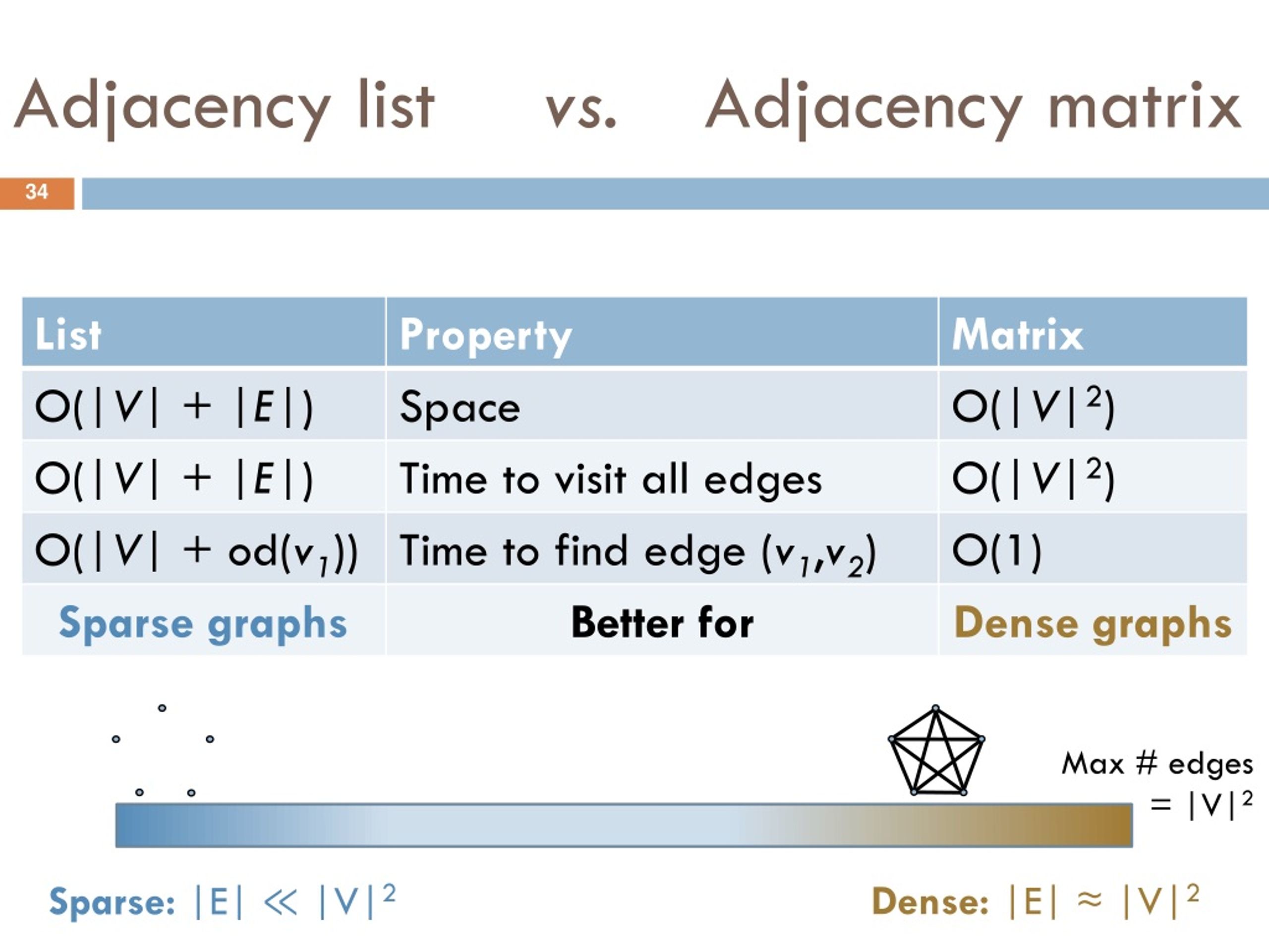
- Adjacency Matrix: The space complexity is always , where is the number of vertices. You need to store a value for every possible pair of vertices, whether an edge exists or not.
- Adjacency List: The space complexity is , where is the number of edges. You store each vertex once, and each edge is represented twice in the lists (for an undirected graph).
This leads to a crucial distinction:
- Sparse Graph: A graph with very few edges. Formally, is much smaller than (e.g., is on the order of ). Social networks are typically sparse; most people are not friends with most other people. For sparse graphs, an adjacency list is far more space-efficient.
- Dense Graph: A graph with many edges, where approaches . A graph where every city is connected to every other city would be dense. For dense graphs, the space of the matrix is comparable to , so the space penalty is minimal.
Metaphor: The Flight Chart vs. The Contact List
If you're creating a flight chart (matrix) for every small airport in a country, but only for one tiny airline's routes, the chart will be almost entirely empty. This is a sparse graph, and you've wasted a ton of paper. A simple list of the few routes that exist (adjacency list) would be much better.
However, if you're mapping all possible flights between the 10 busiest airports in the world, the chart will be nearly full. This is a dense graph, and the chart is an efficient, quick-reference tool.
Concept 5: Time Complexity Trade-offs (Operational Performance)
The final piece of the puzzle is analyzing how fast you can perform common operations. This is often the deciding factor in an algorithm design context.
Technical Explanation
Let's compare the time complexities for the most frequent graph operations. The video below provides an excellent and detailed comparison table.
2. Representation of Graphs - Adjacency List, Matrix with Comparison of Space and Time Complexity!
The video 'Representation of Graphs' from Keerti Purswani offers a fantastic, detailed breakdown of the time complexities for various operations.
Watch the summary from 22:56 to 26:32. This section presents a comprehensive table comparing the time complexities for adding/removing vertices/edges, querying edges, and finding neighbors. Focus on understanding the 'why' behind each complexity value.
Here is a summary of the most critical trade-offs:
| Operation | Adjacency Matrix | Adjacency List | Analysis |
|---|---|---|---|
| Check if edge (u, v) exists | Matrix wins. It's a direct lookup at matrix[u][v]. With a list, you must scan the neighbors of u. |
||
| Iterate neighbors of vertex u | List wins. You only iterate through the actual neighbors. The matrix requires iterating through an entire row. | ||
| Add an edge (u, v) | Tie. Both are fast. Matrix sets matrix[u][v] = 1. List appends v to list[u]. |
||
| Remove an edge (u, v) | Matrix wins. It's a simple assignment. With a list, you must first find the edge to remove it. |
Note: refers to the degree of vertex u—the number of edges connected to it.
Test your understanding!
You are designing a system for a social network like Facebook. Which graph representation would you choose? Justify your decision based on the trade-offs of the two most frequent user operations:
- Loading a user's news feed (which requires fetching content from all their friends).
- Checking if you are already friends with another user you just met.
Show answer
The Adjacency List is the superior choice.
- Graph Density: A social network is a sparse graph. The average user has hundreds of friends, not millions. An adjacency matrix would be astronomically large and mostly empty, making it a non-starter due to space constraints.
- News Feed (Iterate Neighbors): This is the most frequent operation. With an adjacency list, its complexity is , which is very fast for a few hundred friends. With an adjacency matrix, it would be , requiring a scan of millions of potential connections just to find the few hundred that exist. The adjacency list is a clear winner here.
- Friendship Check (Check Edge): An adjacency matrix is faster for this ( vs. ). However, the performance of the adjacency list is still excellent ( is very fast for a few hundred friends) and does not justify the massive space cost and the terrible performance for the primary news feed operation.
Conclusion: The massive advantage of the adjacency list for space and neighbor iteration in a sparse graph far outweighs the minor disadvantage in edge-checking time.
Conclusion
You've now mastered the two fundamental ways to represent a graph in memory and, more importantly, the engineering trade-offs that guide your choice. This isn't just academic; making and justifying this decision is a sign of a senior engineer.
Key Takeaways:
- Adjacency Matrix: Best for dense graphs. Its killer feature is the edge existence check. Its main drawback is the rigid space requirement.
- Adjacency List: Best for sparse graphs, which are far more common in the real world. Its killer feature is efficient neighbor iteration and its flexible space usage.
- The Right Answer: In an interview, the best representation "depends on the problem." Your job is to analyze the graph's expected density and the frequency of operations (edge checks vs. neighbor traversals) to make an informed decision. For most interview problems, the adjacency list is the default choice unless a compelling reason exists to use a matrix.
Preview of the Next Lesson:
With our representations in hand, we are ready to start exploring the graph. Our next lesson will cover our first major traversal algorithm: Breadth-First Search (BFS). You'll learn how to implement BFS to systematically explore a graph level by level, a technique that is the key to finding the shortest path in unweighted graphs.