BFS for Shortest Paths in Unweighted Graphs

The Five Concepts for Today

We will break down BFS into five interrelated concepts, moving from the high-level idea to a complete, interview-ready implementation:

1. The Core Idea of BFS: Exploring in concentric layers.
2. The Shortest Path Property: Why BFS guarantees the shortest path in unweighted graphs.
3. Implementing BFS Traversal: The mechanics of the queue and the visited set.
4. Reconstructing the Shortest Path: Finding the path, not just the destination.
5. Full Implementation and Analysis: A production-ready function and its complexity.

Concept 1: The Core Idea of BFS

Technical Explanation

Breadth-First Search (BFS) is a graph traversal algorithm that starts at a source node and explores all of its immediate neighbors at the present "depth" before moving on to the nodes at the next depth level. This "level-by-level" exploration is the defining characteristic of BFS. To manage this process, BFS relies on two key data structures:

1. A Queue (First-In, First-Out): To keep track of the nodes to visit next. This ensures that we explore nodes in the order they were discovered.
2. A visited Set: To keep track of nodes we have already visited or enqueued, preventing us from processing the same node multiple times and getting trapped in infinite loops in graphs with cycles.

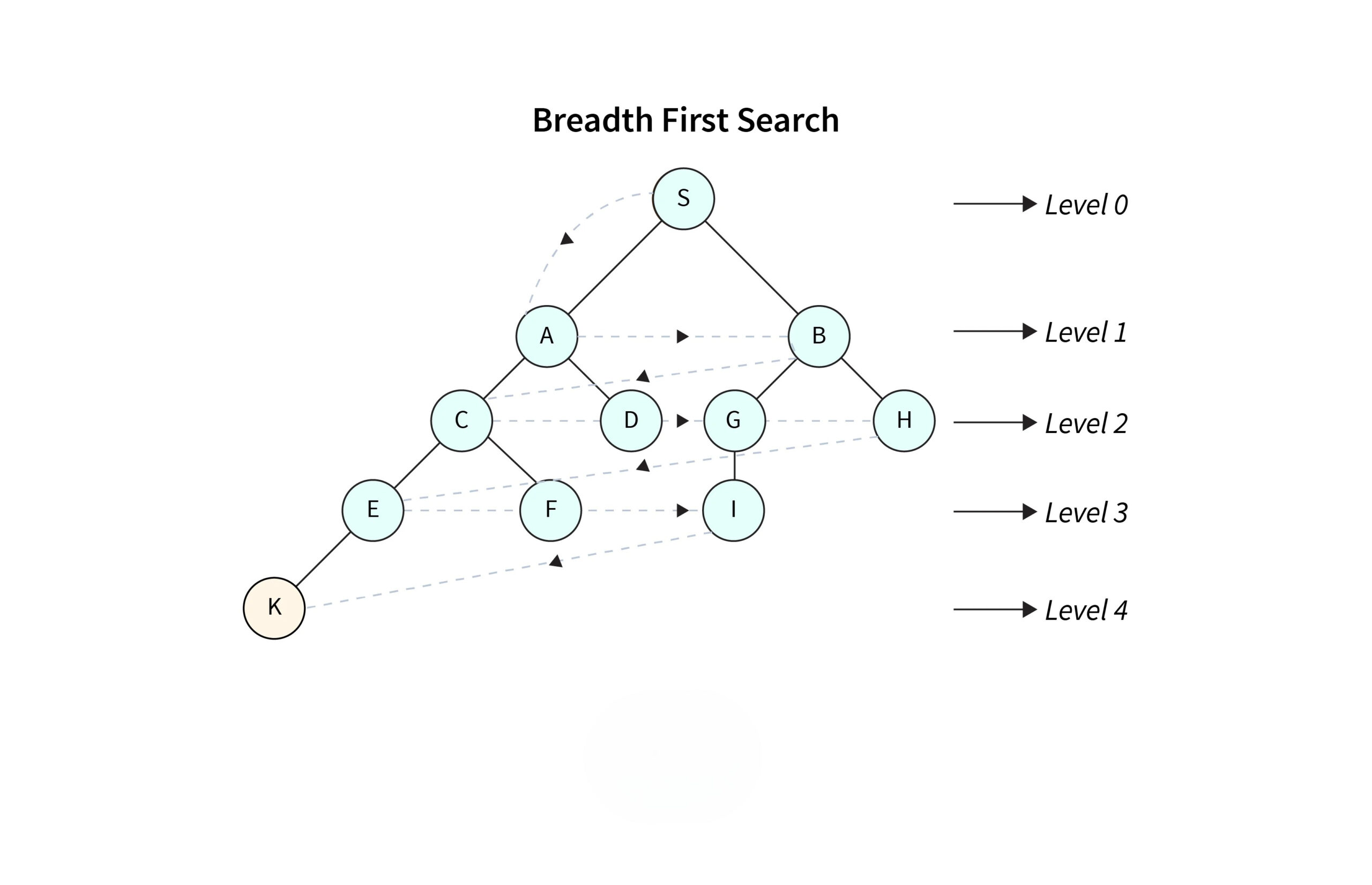
Metaphor: Ripples in a Pond

Imagine dropping a stone into a still pond. The stone is your start node.

• The first ripple that expands outwards represents Level 1: all the nodes directly connected to your start node.
• The second ripple represents Level 2: the neighbors of the Level 1 nodes.
• BFS is like observing these ripples. You fully process the first ripple before you even consider the second. The queue is your mechanism for tracking which parts of the expanding ripple to look at next.

Python Code: Basic Traversal

Here is a barebones implementation of BFS for traversal only. It simply prints the nodes in the order they are visited.

from collections import deque

def bfs_traversal(graph, start_node):
    """
    Performs a BFS traversal of a graph, printing nodes as they are visited.
    
    Args:
        graph (dict): The graph as an adjacency list.
        start_node: The node to begin the traversal from.
    """
    if start_node not in graph:
        print("Start node not in graph.")
        return

    queue = deque([start_node])
    visited = {start_node}
    
    print("BFS Traversal Order:")
    while queue:
        # Dequeue the next node to visit
        current_node = queue.popleft()
        print(current_node, end=" ")
        
        # Enqueue all unvisited neighbors
        for neighbor in graph.get(current_node, []):
            if neighbor not in visited:
                visited.add(neighbor)
                queue.append(neighbor)
    print()

# Example usage:
graph_example = {
    'A': ['B', 'C'],
    'B': ['A', 'D', 'E'],
    'C': ['A', 'F'],
    'D': ['B'],
    'E': ['B', 'F'],
    'F': ['C', 'E']
}
bfs_traversal(graph_example, 'A')
# Expected Output: A B C D E F 

Concept 2: The "Shortest Path" Property

Technical Explanation

The single most important application of BFS is finding the shortest path between two nodes in an unweighted graph. The "shortest path" here means the path with the fewest number of edges.

The level-by-level exploration guarantees this property. When BFS expands from a source s, it first discovers all nodes at distance 1, then all nodes at distance 2, and so on. Therefore, the first time BFS reaches a target node t, it must have done so via a path of the minimum possible length. If a shorter path existed, BFS would have discovered t on an earlier level, which is a contradiction.

This is the central "under the hood" reason why BFS is the right tool for this job, whereas an algorithm like Depth-First Search (DFS) makes no such guarantee.

Metaphor: The Closest Coffee Shop

You're standing at an intersection in a city grid where all blocks are the same length (an unweighted graph). You want to find the absolute closest coffee shop.

• First, you scan all the shops on the same street, 1 block away (Level 1).
• If you don't find one, you systematically check all shops that are exactly 2 blocks away (Level 2).
• You continue this, expanding your search radius by one block at a time.
  The very first coffee shop you find is, by definition, the closest one. You don't need to check any further because any other shop would have to be at the same distance or farther away. BFS operates on this exact principle.

Concept 3: Implementing BFS Traversal

Technical Explanation

Let's formalize the algorithm from Concept 1. The process is straightforward but requires precision.

1. Initialization:

   • Create a queue and add the start_node. A deque from Python's collections library is ideal because popleft() is an $O(1)$ operation.
   • Create a visited set and add the start_node. This prevents re-visiting and is crucial for correctness and termination.

2. Main Loop:

   • Loop as long as the queue is not empty.
   • Dequeue: Remove the node from the front of the queue. Let's call it current_node.
   • Goal Check: (If finding a path) Check if current_node is the target_node. If so, we're done.
   • Explore Neighbors: Iterate through all neighbors of current_node. For each neighbor:
     • If the neighbor has not been visited, add it to the visited set and enqueue it.

To see this process animated and explained clearly, the following resources are excellent.

Metaphor: The Bureaucratic Explorer

Imagine you're a meticulous explorer mapping a cave system (the graph). You have a strict set of rules:

1. You start in the main chamber (start_node). You put it on your "caves to process" list (the queue) and mark it on your map as "explored" (the visited set).
2. You take the first cave from your list. You stand in it.
3. You look at all tunnels leading out of your current cave. For any tunnel that leads to a chamber you haven't marked on your map yet, you mark it as "explored" and add it to the end of your "caves to process" list.
4. You repeat from step 2 until your list is empty.
   This rigid, FIFO process ensures you map the entire system one "layer" of caves at a time.

Python Code: The Traversal Logic

The following code snippet is a more robust version of the traversal logic, using the get() method to handle nodes with no outgoing edges gracefully.

from collections import deque

def bfs_search(graph, start_node, target_node):
    """
    Checks if a path exists between start_node and target_node using BFS.
    """
    if start_node not in graph:
        return False

    queue = deque([start_node])
    visited = {start_node}

    while queue:
        current_node = queue.popleft()

        if current_node == target_node:
            print(f"Path found to {target_node}!")
            return True

        for neighbor in graph.get(current_node, []):
            if neighbor not in visited:
                visited.add(neighbor)
                queue.append(neighbor)
    
    print(f"No path found to {target_node}.")
    return False

# Example usage:
bfs_search(graph_example, 'A', 'F') # Expected: Path found to F!
bfs_search(graph_example, 'A', 'Z') # Expected: No path found to Z.

Concept 4: Reconstructing the Shortest Path

Technical Explanation

The previous code can tell us if a path exists, but it doesn't tell us what the path is. To reconstruct the path, we need to store "breadcrumbs." We use a parent dictionary (or hash map) for this.

The rule is simple: when we discover a neighbor from current_node, we record it: parent[neighbor] = current_node.

Once the BFS reaches the target_node, we can backtrack from the target to the source using this parent map. Starting with the target, we repeatedly look up its parent, then its parent's parent, and so on, until we reach the start_node (whose parent will be None). The sequence of nodes we collect, when reversed, gives us the shortest path.

Metaphor: Ariadne's Thread

This technique is like the Greek myth of Theseus and the Minotaur. To navigate the labyrinth (the graph), Ariadne gave Theseus a ball of thread (the parent map). He unrolled it as he went deeper. After defeating the Minotaur (reaching the target_node), he simply followed the thread back to the entrance (start_node). Our parent map is that magical thread.

Python Code: Adding the Parent Map

Let's modify our BFS to include the parent map.

from collections import deque

def bfs_with_parent_map(graph, start_node, target_node):
    queue = deque([start_node])
    visited = {start_node}
    # Parent map to reconstruct the path
    parent = {start_node: None}

    path_found = False
    while queue:
        current_node = queue.popleft()
        if current_node == target_node:
            path_found = True
            break # Found the target, no need to search further

        for neighbor in graph.get(current_node, []):
            if neighbor not in visited:
                visited.add(neighbor)
                parent[neighbor] = current_node # <-- The crucial step!
                queue.append(neighbor)

    # Now, reconstruct the path by backtracking
    if path_found:
        path = []
        curr = target_node
        while curr is not None:
            path.append(curr)
            curr = parent[curr]
        # The path is from target to source, so we reverse it
        return path[::-1]
    
    return None # No path found

# Example Usage:
path = bfs_with_parent_map(graph_example, 'A', 'F')
print(f"Shortest path from A to F: {path}") 
# Expected Output: Shortest path from A to F: ['A', 'C', 'F'] or ['A', 'B', 'E', 'F']
# Note: ['A', 'C', 'F'] is shorter (2 edges), so it should be found first.
# Let's adjust the example to make the path unambiguous.
graph_example_2 = {'A': ['B', 'C'], 'B': ['D'], 'C': ['E'], 'D': ['F'], 'E':['F'], 'F':[]}
path2 = bfs_with_parent_map(graph_example_2, 'A', 'F')
print(f"Shortest path from A to F: {path2}")
# Expected Output: Shortest path from A to F: ['A', 'B', 'D', 'F']

Concept 5: Full Implementation and Analysis

Technical Explanation

Now, let's assemble everything into a final, robust function. This function will be self-contained and handle edge cases like the start or target not being in the graph, or no path existing.

Time Complexity: The time complexity of BFS is $O(V+E)$, where $V$ is the number of vertices and $E$ is the number of edges. This is because, in the worst case, we visit every vertex once and inspect every edge once.

• Each vertex is enqueued and dequeued exactly once: $O(V)$.
• We iterate through the adjacency list of each vertex once over the entire execution: $O(E)$.

Space Complexity: The space complexity is $O(V)$. This is determined by the maximum size of the data structures we use:

• The visited set can store up to $V$ vertices.
• The parent map can store up to $V$ entries.
• The queue in the worst case (a star-like graph where the center connects to all other $V-1$ nodes) can hold up to $V-1$ nodes at once.

This efficiency makes BFS a highly practical algorithm for large graphs.

Real-World Applications & Interview Questions

• GPS Navigation: Finding the route with the fewest turns (unweighted edges).
• Social Networks: Finding how many "degrees of separation" are between two people (e.g., LinkedIn's 1st, 2nd, 3rd+ connections).
• Web Crawlers: Google bots explore the web level by level starting from a set of root pages.
• Interview Problem Pattern: Many LeetCode problems like "Rotting Oranges," "Word Ladder," or finding the shortest path in a binary matrix are cleverly disguised BFS problems. The "state" (e.g., the current word, the coordinates of an orange) is a node, and a valid transformation (changing one letter, moving to an adjacent cell) is an edge.

Python Code: The Final Function

from collections import deque

def find_shortest_path_bfs(graph: dict, start_node, target_node):
    """
    Finds the shortest path in an unweighted graph using BFS.

    Args:
        graph: The graph represented as an adjacency list.
        start_node: The starting node.
        target_node: The target node.

    Returns:
        A list representing the shortest path, or None if no path exists.
    """
    if start_node not in graph or target_node not in graph:
        return None  # Or raise an error, depending on desired behavior

    queue = deque([start_node])
    visited = {start_node}
    parent = {start_node: None}

    while queue:
        current_node = queue.popleft()

        if current_node == target_node:
            # Reconstruct and return the path
            path = []
            curr = target_node
            while curr is not None:
                path.append(curr)
                curr = parent[curr]
            return path[::-1]  # Reverse to get path from start to target

        for neighbor in graph.get(current_node, []):
            if neighbor not in visited:
                visited.add(neighbor)
                parent[neighbor] = current_node
                queue.append(neighbor)
    
    return None # Target was not reachable

# Final test with our graph
final_path = find_shortest_path_bfs(graph_example_2, 'A', 'F')
if final_path:
    print(f"The shortest path has {len(final_path) - 1} edges: {final_path}")
else:
    print("No path was found.")

Conclusion

Today, you've moved beyond static graph representations to dynamic traversal. You implemented Breadth-First Search, a fundamental algorithm for exploring a graph and, crucially, for finding the shortest path in an unweighted context.

Key Takeaways:

• BFS explores level by level using a queue (FIFO).
• This level-order exploration naturally guarantees the shortest path in terms of the number of edges.
• An implementation requires a queue for managing nodes to visit and a visited set to avoid cycles and redundant work.
• To reconstruct the path, you need a parent map to store "breadcrumbs" and backtrack from the target to the source.
• The algorithm is highly efficient, with $O(V+E)$ time complexity and $O(V)$ space complexity.

Preview of the Next Lesson:
We've explored broadly; next, we'll explore deeply. Our next lesson introduces Depth-First Search (DFS). While BFS uses a queue to stay shallow, DFS uses a stack (often implicitly via recursion) to dive as deep as possible down one path before backtracking. We'll implement it both recursively and iteratively and begin to analyze the very different types of problems for which DFS is the ideal tool, such as cycle detection and topological sorting.