Knapsack and Subset Sum Problems

Today's Concepts

1. Defining the 0/1 Knapsack Problem
2. The 2D DP Solution for 0/1 Knapsack
3. The Subset Sum Problem: A Knapsack Variation
4. Backtracking to Find the Optimal Set
5. Complexity, Optimizations, and Real-World Impact

Concept 1: Defining the 0/1 Knapsack Problem

Let's begin by formally understanding the problem we're trying to solve. It's a cornerstone of combinatorial optimization.

Technical Explanation

The 0/1 Knapsack Problem gives you:

1. A set of n items, where each item i has a weight $w_i$ and a value $v_i$.
2. A knapsack with a maximum weight capacity $C$.

The goal is to choose a subset of items to put into the knapsack such that the total value is maximized, and the total weight does not exceed the capacity $C$. The "0/1" constraint means that for each item, you have a binary choice: you either take the whole item (1) or you leave it behind (0). You cannot take a fraction of an item.

The decision for each item creates a branching path of possibilities, making it a perfect candidate for dynamic programming.

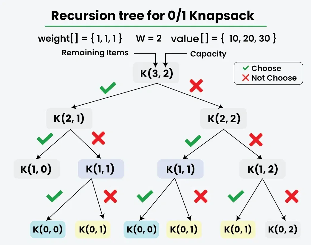
Metaphor: The Elite Coder's Dilemma

Imagine you're at a tech conference with a limited-edition swag bag that can only hold 5kg. You're at a sponsor's booth with amazing loot:

• A mechanical keyboard: weight=2kg, value (to you)=9/10
• A high-end GPU: weight=4kg, value=10/10
• A collection of programming books: weight=3kg, value=7/10

You can't take everything. Taking the GPU (4kg) leaves you with only 1kg of capacity, so you can't get anything else. Taking the keyboard (2kg) and the books (3kg) perfectly fills your bag for a total value of 16/10. This is the better choice. The 0/1 Knapsack algorithm is the systematic process you'd use to make this optimal decision, especially if there were hundreds of items.

Concept 2: The 2D DP Solution for 0/1 Knapsack

Just as we used a 2D grid for LCS, we'll use a 2D table to solve the 0/1 Knapsack problem. The key is defining the state correctly.

Technical Explanation

We'll construct a 2D table, dp, of size (n+1) x (C+1), where n is the number of items and C is the knapsack capacity.

• State Definition: dp[i][w] will store the maximum value we can achieve using a subset of the first i items with a knapsack capacity of exactly w.

• Recurrence Relation: To compute dp[i][w], we consider the i-th item (with value[i-1] and weight[i-1]). We have two choices:

  1. Don't include item i: If we don't take the i-th item, the maximum value we can get is simply the best we could do with the first i-1 items and the same capacity w.
     $\text{value\_if\_excluded}=dp[i-1][w]$

  2. Include item i: We can only do this if weight[i-1] <= w. If we include it, we gain value[i-1], but we must use up weight[i-1] of our capacity. The remaining value comes from the best we could do with the first i-1 items and the remaining capacity w - weight[i-1].
     $\text{value\_if\_included}=value[i-1]+dp[i-1][w-weight[i-1]]$

  Since we want to maximize value, we take the best of these two options.

  $$dp[i][w]=\max (dp[i-1][w],value[i-1]+dp[i-1][w-weight[i-1]])$$

  If the item is too heavy to be included (weight[i-1] > w), we are forced to exclude it, so dp[i][w] = dp[i-1][w].

• Base Cases: dp[0][w] = 0 for all w (no items, no value), and dp[i][0] = 0 for all i (no capacity, no value). The final answer is dp[n][C].

The following video provides a masterful walkthrough of this entire process.

Implementation (Tabulation)

Here is the Python implementation of the bottom-up approach.

def knapsack_01(values, weights, capacity):
    """
    Solves the 0/1 Knapsack problem using 2D Dynamic Programming.
    Time Complexity: O(n * C)
    Space Complexity: O(n * C)
    """
    n = len(values)
    # dp[i][w] = max value using first i items with capacity w
    dp = [[0] * (capacity + 1) for _ in range(n + 1)]

    for i in range(1, n + 1):
        # Current item's index in original arrays is i-1
        current_value = values[i-1]
        current_weight = weights[i-1]
        for w in range(1, capacity + 1):
            # If the current item is too heavy, we must exclude it.
            if current_weight > w:
                dp[i][w] = dp[i-1][w]
            else:
                # Decide whether to include or exclude the current item
                value_if_excluded = dp[i-1][w]
                value_if_included = current_value + dp[i-1][w - current_weight]
                dp[i][w] = max(value_if_included, value_if_excluded)
    
    return dp[n][capacity]

# Example from the metaphor
values = [9, 10, 7]
weights = [2, 4, 3]
capacity = 5
max_val = knapsack_01(values, weights, capacity)
print(f"Maximum value for the swag bag: {max_val}") # Expected: 16 (keyboard + books)

Concept 3: The Subset Sum Problem: A Knapsack Variation

The Subset Sum problem is a classic decision problem that can be elegantly solved using the logic we just developed for the knapsack problem.

Technical Explanation

Problem: Given a set of non-negative integers and a target sum S, determine if there exists a subset of the given set whose elements sum up to S.

This is a decision problem ("yes" or "no"), not an optimization problem. We can frame it as a 0/1 Knapsack problem where for each item, its value is equal to its weight. The question then becomes: "Is it possible to achieve a total 'value' of exactly S with a 'knapsack capacity' of S?"

• State Definition: dp[i][j] will be a boolean value indicating whether a sum of j can be achieved using a subset of the first i numbers.

• Recurrence Relation: For each number num[i-1], we have two choices:

  1. Don't include num[i-1]: The possibility of making sum j depends only on whether it was possible with the first i-1 numbers: dp[i-1][j].
  2. Include num[i-1]: We can do this if num[i-1] <= j. The possibility depends on whether we could form the remaining sum, j - num[i-1], with the first i-1 numbers: dp[i-1][j - num[i-1]].

  Since we just need to know if either path is possible, we use a logical OR.

  $$dp[i][j]=dp[i-1][j]\vee dp[i-1][j-\text{num}[i-1]]$$

Implementation

The following resource provides a detailed look at solving Subset Sum with DP.

def subset_sum(nums, target_sum):
    """
    Solves the Subset Sum problem using 2D Dynamic Programming.
    Time Complexity: O(n * S)
    Space Complexity: O(n * S)
    """
    n = len(nums)
    # dp[i][j] = True if sum j is possible with first i numbers
    dp = [[False] * (target_sum + 1) for _ in range(n + 1)]

    # Base case: a sum of 0 is always possible (with an empty set)
    for i in range(n + 1):
        dp[i][0] = True

    for i in range(1, n + 1):
        current_num = nums[i-1]
        for j in range(1, target_sum + 1):
            # If the current number is larger than the target sum j, we must exclude it.
            if current_num > j:
                dp[i][j] = dp[i-1][j]
            else:
                # It's possible if we could either make the sum without this number,
                # OR if we could make the remaining sum (j - current_num) before.
                dp[i][j] = dp[i-1][j] or dp[i-1][j - current_num]

    return dp[n][target_sum]

nums = [3, 34, 4, 12, 5, 2]
target = 9
print(f"Is a subset with sum {target} possible? {subset_sum(nums, target)}") # Expected: True

Concept 4: Backtracking to Find the Optimal Set

The DP table gives us the maximum value (for Knapsack) or a boolean answer (for Subset Sum), but it doesn't tell us which items constitute the solution. We can find this by backtracking through the filled table.

Technical Explanation

The logic is to retrace the decisions made to fill the table, starting from the final cell dp[n][C].

1. Start at i = n and w = C (or j = S for Subset Sum).
2. Compare the value of the current cell dp[i][w] with the cell directly above it, dp[i-1][w].
   • If dp[i][w] == dp[i-1][w]: This means the optimal solution at this point did not include item i. So, we move up to the previous row: i = i - 1.
   • If dp[i][w] != dp[i-1][w]: This implies that item i was included to achieve this optimal value. We add item i to our solution set. Then, we move up to the previous row i = i - 1 and also move left by the item's weight to account for the capacity it used: w = w - weight[i-1].
3. Repeat this process until i or w becomes 0.

Metaphor: Following the Breadcrumbs

Imagine the filled DP table is a map of a maze you've already solved. You're standing at the exit (dp[n][C]). To find your way back to the entrance, you check your path. At each step i, you ask: "Did my score increase when I went from row i-1 to row i?" If it didn't, it means you took a path that ignored item i. If it did, you took the path that included item i, so you mark it on your map and adjust your position accordingly. You're following the "breadcrumbs" of increasing value back to the start.

W3Schools has a great visual guide for this process. In their article DSA The 0/1 Knapsack Problem, the section "Which Items Gives Us The Highest Value?" provides a step-by-step walkthrough with a diagram showing how to trace back the solution.

Implementation (Augmenting the Knapsack Code)

def knapsack_01_with_items(values, weights, capacity):
    n = len(values)
    dp = [[0] * (capacity + 1) for _ in range(n + 1)]

    for i in range(1, n + 1):
        val, wt = values[i-1], weights[i-1]
        for w in range(1, capacity + 1):
            if wt > w:
                dp[i][w] = dp[i-1][w]
            else:
                dp[i][w] = max(dp[i-1][w], val + dp[i-1][w - wt])
    
    # --- Backtracking phase ---
    max_value = dp[n][capacity]
    included_items = []
    w = capacity
    for i in range(n, 0, -1):
        # If the value is the same as the row above, this item was not included.
        if dp[i][w] == dp[i-1][w]:
            continue
        else:
            # This item must have been included.
            included_items.append(values.index(values[i-1])) # appending index
            w -= weights[i-1]
            
    included_items.reverse() # Items are found from last to first
    return max_value, included_items

values = [60, 100, 120]
weights = [10, 20, 30]
capacity = 50
max_val, items = knapsack_01_with_items(values, weights, capacity)
print(f"Max value: {max_val}, Items (by index): {items}") # Expected: 220, [1, 2]

Concept 5: Complexity, Optimizations, and Real-World Impact

Understanding the performance characteristics of these algorithms is critical for interviews.

Time Complexity and Pseudo-Polynomial Time

For both 0/1 Knapsack and Subset Sum, the time complexity is $O(n\cdot C)$, where n is the number of items and C is the capacity/target sum. This is because we fill a table of size (n+1) x (C+1).

This leads to a crucial concept: pseudo-polynomial time. The runtime depends not just on the number of inputs (n), but on the magnitude of an input value (C). If C is a reasonably sized number (e.g., in the thousands), this is very efficient. But if C is extremely large (e.g., 2^n), the runtime becomes exponential in the number of bits needed to represent C, and the algorithm is no longer efficient. Being able to discuss this distinction shows a deep level of understanding.

Space Optimization

In our 2D DP table, notice that the calculation for row i (dp[i]) only ever depends on the results from row i-1. We don't need the entire n x C table in memory at once. We can optimize the space complexity from O(n \cdot C) to O(C) by using only two rows (a current row and a previous row) or even just a single 1D array.

Here is the space-optimized version for Subset Sum:

def subset_sum_optimized(nums, target_sum):
    """
    Solves Subset Sum with O(S) space complexity.
    """
    dp = [False] * (target_sum + 1)
    dp[0] = True # Base case

    for num in nums:
        # We iterate backwards to prevent using the same item multiple times in one pass
        for j in range(target_sum, num - 1, -1):
            dp[j] = dp[j] or dp[j - num]
            
    return dp[target_sum]

nums = [3, 34, 4, 12, 5, 2]
target = 9
print(f"Is a subset with sum {target} possible (optimized)? {subset_sum_optimized(nums, target)}")

Real-World Applications

• 0/1 Knapsack:
  • Cloud Resource Allocation: Choosing which virtual machine jobs (with resource 'weights' and monetary 'values') to run on a server with limited CPU/RAM ('capacity').
  • Finance: Selecting a portfolio of projects or investments to fund from a limited budget to maximize expected return.
  • Logistics: Deciding what cargo to load onto a plane or truck to maximize profit without exceeding weight limits.
• Subset Sum:
  • Cryptography: It forms the basis of some cryptographic systems (like the Merkle-Hellman knapsack cryptosystem, although it is now considered insecure).
  • Financial Auditing: Finding a set of transactions that add up to a disputed or fraudulent amount.

Conclusion

Congratulations on tackling the Knapsack family of problems! You've learned how to approach constrained optimization problems and seen how a powerful pattern can be adapted to solve different, yet related, challenges.

Key Takeaways:

• Knapsack Pattern: The core logic is to make a binary choice (include or exclude) for each item, leading to a max() or or in the recurrence relation.
• State Definition is Key: The power of this DP approach lies in defining dp[i][w] as the optimal solution for a prefix of items and a sub-capacity.
• From Optimization to Decision: The Subset Sum problem demonstrated how the knapsack optimization framework can be simplified for "yes/no" decision problems.
• Complexity Matters: The O(n*C) complexity is efficient but has limitations. Understanding its pseudo-polynomial nature and the O(C) space optimization is what separates a good answer from a great one.
• Backtracking for the Solution: The DP table provides the optimal value; backtracking is the standard procedure to find the items that produce it.

Preview of the Next Lesson:
We will continue exploring advanced DP patterns. Our next lesson will focus on problems that involve states represented by bitmasks. DP with Bitmasking is a powerful technique that allows you to solve problems on subsets and permutations that seem intractable at first glance, unlocking a whole new level of problem-solving capability.